Coupled Noises Analysis
Contents
Coupled Noises Analysis#
Due: Febuary 5, 2020
Author: Kevin Egedy
Objectives#
This lab introduces the characteristics of backward and forward coupled noises on coupled transmission lines. You will also study how to obtain the coupling coefficients and lumped element models from the measured data.
# Libraries
#
import sympy as sp
import pandas as pd
import numpy as np
import matplotlib.pyplot as plt
import matplotlib.patches as pch
from helperfunctions import *
%matplotlib inline
from IPython.core.interactiveshell import InteractiveShell
InteractiveShell.ast_node_interactivity = "all"
files = [
    'LineA_Ch1Reflection_2ns_31.6nsOffset',
    'LineA_Ch1Reflection_OPEN_2ns_30nsOffset',
    'LineA_ChA_OPEN_500ps_41.75nsOffset',
    'LineA_ChA_SHORT_500ps_41.750nsOffset',
    'LineA_ChB_OPEN_500ps_41.75nsOffset',
    'LineA_ChB_SHORT_500ps_41.952nsOffset',
    'LineB_Ch1Reflection_1200ps_33.9808nsOffset',
    'LineB_Ch1Reflection_OPEN_2ns_30nsOffset',
    'LineB_ChA_OPEN_500ps_41nsOffset',
    'LineB_ChA_SHORT_1080ps_41.0184nsOffset',
    'LineB_ChB_OPEN_500ps_41.75nsOffset',
    'LineB_ChB_SHORT_600ps_41.952nsOffset',
    'LineC_Ch1Reflection_2.4ns_30.91nsOffset',
    'LineC_Ch1Reflection_OPEN_2ns_30nsOffset',
    'LineC_ChA_OPEN_500ps_41.75nsOffset',
    'LineC_ChA_SHORT_490ps_41.38nsOffset',
    'LineC_ChB_OPEN_500ps_41.75nsOffset',
    'LineC_ChB_SHORT_430ps_42nsOffset'
]
%%capture
# Read .xlsx files and convert them into .csv
#
for filename in files:
    df = pd.read_excel(f'data/{filename}.xlsx',header=None,nrows=1)
    with open(f'data/csv/{filename}.csv','w+') as f0:
        f0.write(df.T.to_csv(index=False,header=None));
# Read .csv files into numpy arrays
#
LineA_Ch1Reflection_2ns_31 = \
  pd.read_csv('data/csv/LineA_Ch1Reflection_2ns_31.6nsOffset.csv',
    header=None).to_numpy()

LineA_Ch1Reflection_OPEN_2ns_30 = \
  pd.read_csv('data/csv/LineA_Ch1Reflection_OPEN_2ns_30nsOffset.csv',
    header=None).to_numpy()

LineA_ChA_OPEN_500ps_41 = \
  pd.read_csv('data/csv/LineA_ChA_OPEN_500ps_41.75nsOffset.csv',
    header=None).to_numpy()

LineA_ChA_SHORT_500ps_41 = \
  pd.read_csv('data/csv/LineA_ChA_SHORT_500ps_41.750nsOffset.csv',
    header=None).to_numpy()

LineA_ChB_OPEN_500ps_41 = \
  pd.read_csv('data/csv/LineA_ChB_OPEN_500ps_41.75nsOffset.csv',
    header=None).to_numpy()

LineA_ChB_SHORT_500ps_41 = \
  pd.read_csv('data/csv/LineA_ChB_SHORT_500ps_41.952nsOffset.csv',
    header=None).to_numpy()

LineB_Ch1Reflection_1200ps_33 = \
  pd.read_csv('data/csv/LineB_Ch1Reflection_1200ps_33.9808nsOffset.csv',
    header=None).to_numpy()

LineB_Ch1Reflection_OPEN_2ns_30 = \
  pd.read_csv('data/csv/LineB_Ch1Reflection_OPEN_2ns_30nsOffset.csv',
    header=None).to_numpy()

LineB_ChA_OPEN_500ps_41 = \
  pd.read_csv('data/csv/LineB_ChA_OPEN_500ps_41nsOffset.csv',
    header=None).to_numpy()

LineB_ChA_SHORT_1080ps_41 = \
  pd.read_csv('data/csv/LineB_ChA_SHORT_1080ps_41.0184nsOffset.csv',
    header=None).to_numpy()

LineB_ChB_OPEN_500ps_41 = \
  pd.read_csv('data/csv/LineB_ChB_OPEN_500ps_41.75nsOffset.csv',
    header=None).to_numpy()

LineB_ChB_SHORT_600ps_41 = \
  pd.read_csv('data/csv/LineB_ChB_SHORT_600ps_41.952nsOffset.csv',
    header=None).to_numpy()

LineC_Ch1Reflection_2ns_30 = \
  pd.read_csv('data/csv/LineC_Ch1Reflection_2.4ns_30.91nsOffset.csv',
    header=None).to_numpy()

LineC_Ch1Reflection_OPEN_2ns_30 = \
  pd.read_csv('data/csv/LineC_Ch1Reflection_OPEN_2ns_30nsOffset.csv',
    header=None).to_numpy()

LineC_ChA_OPEN_500ps_41 = \
  pd.read_csv('data/csv/LineC_ChA_OPEN_500ps_41.75nsOffset.csv',
    header=None).to_numpy()

LineC_ChA_SHORT_490ps_41 = \
  pd.read_csv('data/csv/LineC_ChA_SHORT_490ps_41.38nsOffset.csv',
    header=None).to_numpy()

LineC_ChB_OPEN_500ps_41 = \
  pd.read_csv('data/csv/LineC_ChB_OPEN_500ps_41.75nsOffset.csv',
    header=None).to_numpy()

LineC_ChB_SHORT_430ps_42 = \
  pd.read_csv('data/csv/LineC_ChB_SHORT_430ps_42nsOffset.csv',
    header=None).to_numpy()
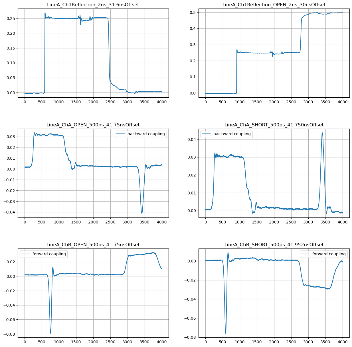
# Plot Overview LineA
#
fig,axs = plt.subplots(3,2,figsize=(15,15))
plt.subplots_adjust(hspace=0.35)
plt.subplots_adjust(wspace=0.20)

axs[0,0].plot(LineA_Ch1Reflection_2ns_31)
axs[0,1].plot(LineA_Ch1Reflection_OPEN_2ns_30)
axs[1,0].plot(LineA_ChA_OPEN_500ps_41,label='backward coupling')
axs[1,1].plot(LineA_ChA_SHORT_500ps_41,label='backward coupling')
axs[2,0].plot(LineA_ChB_OPEN_500ps_41,label='forward coupling')
axs[2,1].plot(LineA_ChB_SHORT_500ps_41,label='forward coupling')

axs[0,0].set_title('LineA_Ch1Reflection_2ns_31.6nsOffset')
axs[0,1].set_title('LineA_Ch1Reflection_OPEN_2ns_30nsOffset')
axs[1,0].set_title('LineA_ChA_OPEN_500ps_41.75nsOffset')
axs[1,1].set_title('LineA_ChA_SHORT_500ps_41.750nsOffset')
axs[2,0].set_title('LineA_ChB_OPEN_500ps_41.75nsOffset')
axs[2,1].set_title('LineA_ChB_SHORT_500ps_41.952nsOffset')

axs[0,0].grid(True)
axs[0,1].grid(True)
axs[1,0].grid(True)
axs[1,1].grid(True)
axs[2,0].grid(True)
axs[2,1].grid(True)

axs[1,0].legend()
axs[1,1].legend()
axs[2,0].legend()
axs[2,1].legend();
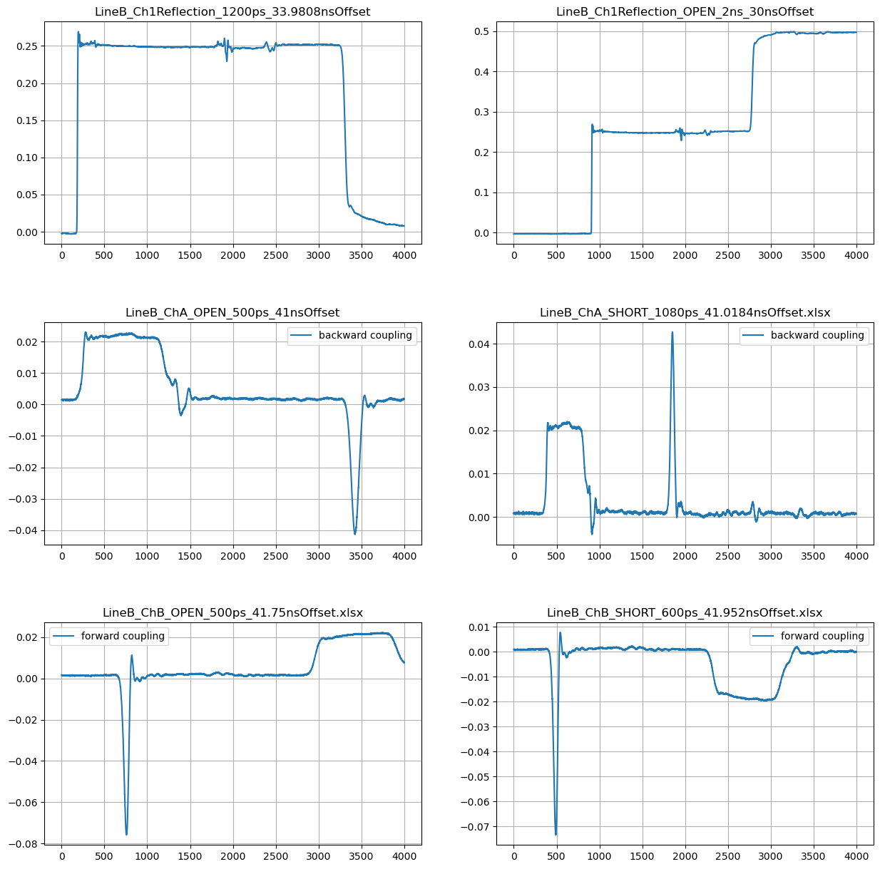
# Plot Overview LineB
#
fig,axs = plt.subplots(3,2,figsize=(15,15))
plt.subplots_adjust(hspace=0.35)
plt.subplots_adjust(wspace=0.20)

axs[0,0].plot(LineB_Ch1Reflection_1200ps_33)
axs[0,1].plot(LineB_Ch1Reflection_OPEN_2ns_30)
axs[1,0].plot(LineB_ChA_OPEN_500ps_41,label='backward coupling')
axs[1,1].plot(LineB_ChA_SHORT_1080ps_41,label='backward coupling')
axs[2,0].plot(LineB_ChB_OPEN_500ps_41,label='forward coupling')
axs[2,1].plot(LineB_ChB_SHORT_600ps_41,label='forward coupling')

axs[0,0].set_title('LineB_Ch1Reflection_1200ps_33.9808nsOffset')
axs[0,1].set_title('LineB_Ch1Reflection_OPEN_2ns_30nsOffset')
axs[1,0].set_title('LineB_ChA_OPEN_500ps_41nsOffset')
axs[1,1].set_title('LineB_ChA_SHORT_1080ps_41.0184nsOffset.xlsx')
axs[2,0].set_title('LineB_ChB_OPEN_500ps_41.75nsOffset.xlsx')
axs[2,1].set_title('LineB_ChB_SHORT_600ps_41.952nsOffset.xlsx')

axs[0,0].grid(True)
axs[0,1].grid(True)
axs[1,0].grid(True)
axs[1,1].grid(True)
axs[2,0].grid(True)
axs[2,1].grid(True)

axs[1,0].legend()
axs[1,1].legend()
axs[2,0].legend()
axs[2,1].legend();
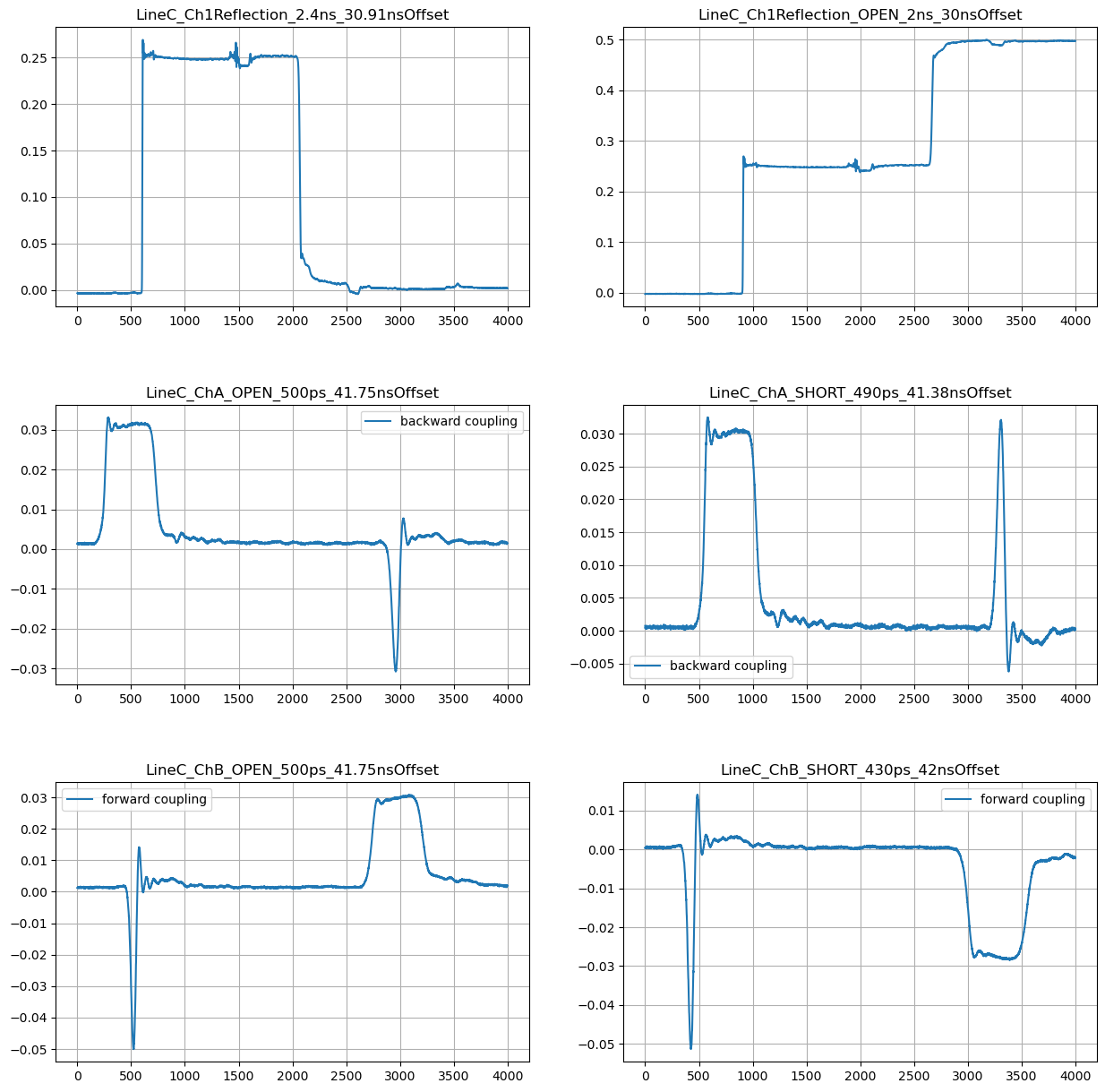
# Plot Overview LineC
#
fig,axs = plt.subplots(3,2,figsize=(15,15))
plt.subplots_adjust(hspace=0.35)
plt.subplots_adjust(wspace=0.20)

axs[0,0].plot(LineC_Ch1Reflection_2ns_30)
axs[0,1].plot(LineC_Ch1Reflection_OPEN_2ns_30)
axs[1,0].plot(LineC_ChA_OPEN_500ps_41,label='backward coupling')
axs[1,1].plot(LineC_ChA_SHORT_490ps_41,label='backward coupling')
axs[2,0].plot(LineC_ChB_OPEN_500ps_41,label='forward coupling')
axs[2,1].plot(LineC_ChB_SHORT_430ps_42,label='forward coupling')

axs[0,0].set_title('LineC_Ch1Reflection_2.4ns_30.91nsOffset')
axs[0,1].set_title('LineC_Ch1Reflection_OPEN_2ns_30nsOffset')
axs[1,0].set_title('LineC_ChA_OPEN_500ps_41.75nsOffset')
axs[1,1].set_title('LineC_ChA_SHORT_490ps_41.38nsOffset')
axs[2,0].set_title('LineC_ChB_OPEN_500ps_41.75nsOffset')
axs[2,1].set_title('LineC_ChB_SHORT_430ps_42nsOffset')

axs[0,0].grid(True)
axs[0,1].grid(True)
axs[1,0].grid(True)
axs[1,1].grid(True)
axs[2,0].grid(True)
axs[2,1].grid(True)

axs[1,0].legend()
axs[1,1].legend()
axs[2,0].legend()
axs[2,1].legend();
Constants#
Permittivity of free-space \(= \epsilon_0 = 8.854 \cdot 10^{-12} F/m\)
Permeability of free-space \(= \mu_0 = 4\pi \cdot 10^{-7} H/m\)
Impedance of free-space \(= \eta_0 = 120\pi = 376.7\Omega\)
Velocity of light in free-space \(= c = 2.998 \cdot 10^8 m/s\)
Notes#
signal duration: \([V_{in}(t) - V_{in}(t-\frac{2d}{v_0})]\)
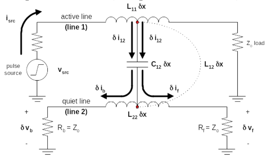
Coupling Coefficient
\(K_C\): capacitive coupling coefficient
\(K_L\): inductive coupling coefficient
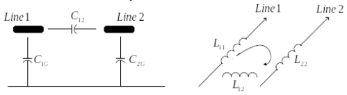
\(\begin{eqnarray} K_C &=& \frac{C_{12}}{C_{1G}+C_{12}} \\[0.5em] K_L &=& \frac{L_{12}}{L_{11}} &&(L_{22} = L_{11}) \end{eqnarray}\)
Coupled Lines |
A |
B |
C |
|---|---|---|---|
Coupled length d (cm) |
10 |
10 |
5 |
Line separation s (mm) |
0.5 |
1 |
0.5 |
Parameter |
units |
Value |
|---|---|---|
\(v_0\) |
m/s |
\(1.71\) \(\cdot\) \(10^8\) |
\(K_C\) (method 1) |
\(0.19890\) |
|
\(K_L\) (method 1) |
\(0.26191\) |
|
\(K_C\) (integration method) |
\(0.19220\) |
|
\(K_L\) (integration method) |
\(0.28164\) |
|
\(Z_{01}\) |
ohms |
\(45.97\) |
\(C_{12}\) |
pF |
\(24.50\) |
\(C_{1G} = C_{2G}\) |
pF |
\(102.77\) |
\(L_{11} = L_{22}\) |
nH |
\(268.80\) |
\(L_{12}\) |
nH |
\(75.71\) |
np_arrays = [
    LineA_Ch1Reflection_2ns_31,         #
    LineA_Ch1Reflection_OPEN_2ns_30,    #
    LineA_ChA_OPEN_500ps_41,            #
    LineA_ChA_SHORT_500ps_41,           #
    LineA_ChB_OPEN_500ps_41,            #
    LineA_ChB_SHORT_500ps_41,           #
    LineB_Ch1Reflection_1200ps_33,      #
    LineB_Ch1Reflection_OPEN_2ns_30,    #
    LineB_ChA_OPEN_500ps_41,            #
    LineB_ChA_SHORT_1080ps_41,          #
    LineB_ChB_OPEN_500ps_41,            #
    LineB_ChB_SHORT_600ps_41,           #
    LineC_Ch1Reflection_2ns_30,         #
    LineC_Ch1Reflection_OPEN_2ns_30,    #
    LineC_ChA_OPEN_500ps_41,            #
    LineC_ChA_SHORT_490ps_41,           #
    LineC_ChB_OPEN_500ps_41,            #
    LineC_ChB_SHORT_430ps_42            #
]
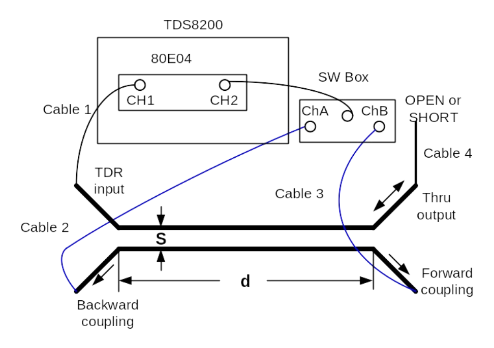
Procedure#
(1) Reflected, Backward and Forward Coupled Noise Measurements
Steps:
Connect the TDR input (Ch1) to the main line (start with the coupled line A)
Connect Ch A to the backward coupled path
Connect Ch B to the forward coupled path
Connect Cable 4 (short black cable) to the transmitted output
Data:
Measure voltage with SHORT connected at the end of Cable 4
Measure voltage with OPEN circuit connected at the end of Cable 4
Repeat the same measurements for coupled lines B and C. Make sure to connect four cables the same way
Line A#
Analysis and Estimation of \(K_C\) and \(K_L\)#
Use Ch 1 data (reflection) for estimating the characteristics impedance of the coupled lines
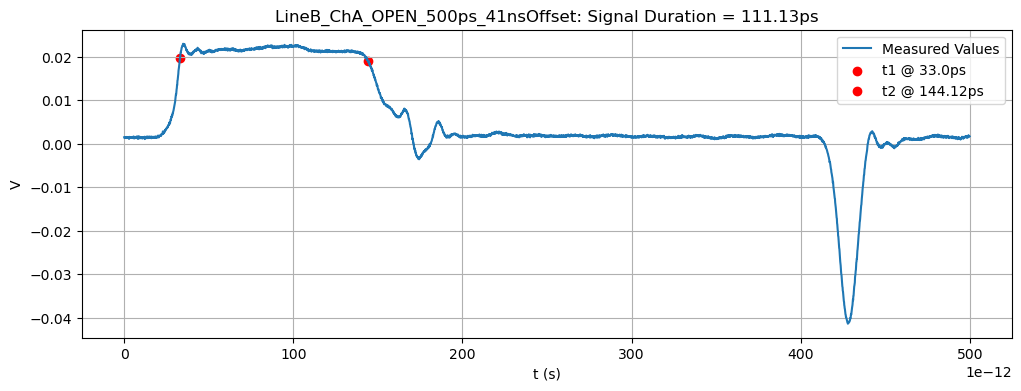
(1) Obtain the signal speed \(v_0\) on the TL using \(V_b\) waveform#
Assume the waveform is a square wave
# Signal Duration: LineA_ChA_OPEN_500ps_41.75nsOffset
#
fig,ax = plt.subplots(figsize=(12,4))
L = len(LineA_ChA_OPEN_500ps_41)
total_time = 500*10**(-12)
mag = 12
unit='ps'
x,res = np.linspace(0,total_time,L,endpoint=False,retstep=True)
Ures = res*10**mag

# Define starting/ending points of input waveform
x10R,x90R = RiseTime( LineA_ChA_OPEN_500ps_41[0:1000] )
x90F,x10F = FallTime( LineA_ChA_OPEN_500ps_41[1000:1500] )
x0 = x90R
x1 = 1000+x90F

# Plot
ax.plot(x,LineA_ChA_OPEN_500ps_41,
    label='Measured Values'
)
ax.scatter(x0*res,LineA_ChA_OPEN_500ps_41[x0],
    color='red',
    label=f't1 @ {round(x0*Ures,2)}{unit}'
)
ax.scatter(x1*res,LineA_ChA_OPEN_500ps_41[x1],
    color='red',
    label=f't2 @ {round(x1*Ures,2)}{unit}'
)

# Labels
rt = RoundNonZeroDecimal((x1*Ures)-(x0*Ures),2)
ax.ticklabel_format(axis='x',style='sci', scilimits=(-mag,-mag))
ax.set_title(f'LineA_ChA_OPEN_500ps_41.75nsOffset: Signal Duration = {rt}{unit}')
ax.set_xlabel('t (s)')
ax.set_ylabel('V')
plt.grid(True)
plt.legend();
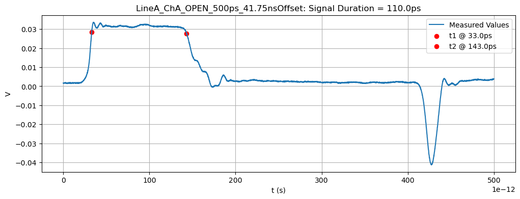
Given: \(d = L = 0.1 \text{m}\)
Measured:
\(\begin{eqnarray} t &=& 110 \text{ps} \end{eqnarray}\)
Solve:
\(\begin{eqnarray} \Delta T &=& \frac{2L}{v} \\ v &=& \frac{2L}{\Delta T} \\ v &=& \frac{2(0.1)}{110 \cdot 10^{-12}} \\ \\ &=& 1.8182 \cdot 10^8 \text{m/s} \end{eqnarray}\)
Signal Speed Summary
Measured signal speed \(v_0\) on the TL using \(V_b\) waveform is \(1.82 \cdot 10^8\) m/s.
Given value is \(1.71 \cdot 10^8\) m/s.
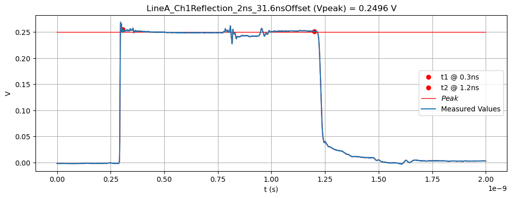
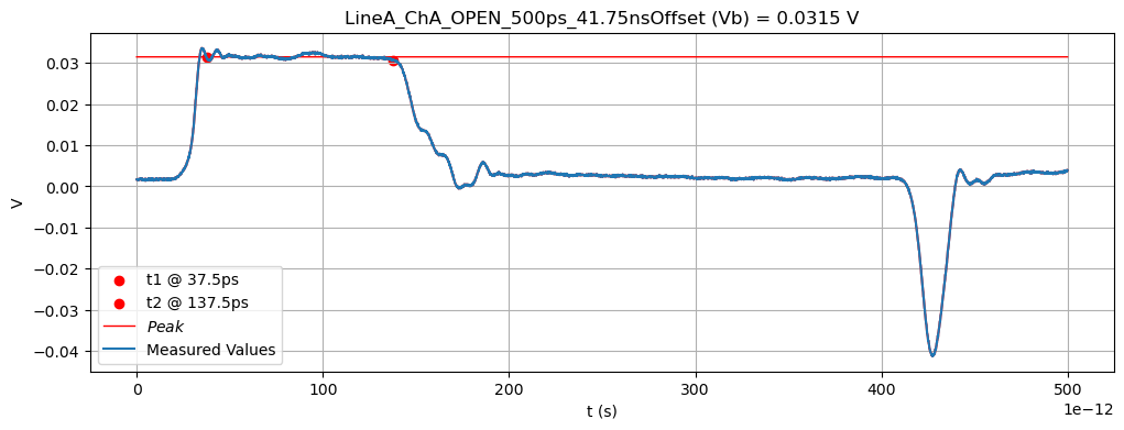
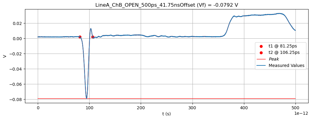
(2) Using the peak values of \(V_b\) and \(V_f\), estimate \(K_C\) and \(K_L\)#
\([V_{in}(t) - V_{in}(t-\frac{2d}{v_0})] \rightarrow V_{\text{peak}}\)
# Vpeak: LineA_Ch1Reflection_2ns_31.6nsOffset
WaveformPeakPlt(
LineA_Ch1Reflection_2ns_31,
x0=610,
x1=2400,
total_time=2*10**(-9),
mag=9,
unit='ns',
title='LineA_Ch1Reflection_2ns_31.6nsOffset (Vpeak)'
)
# Vb: LineA_ChA_OPEN_500ps_41.75nsOffset
WaveformPeakPlt(
LineA_ChA_OPEN_500ps_41,
x0=300,
x1=1100,
total_time=500*10**(-12),
mag=12,
unit='ps',
title='LineA_ChA_OPEN_500ps_41.75nsOffset (Vb)'
)
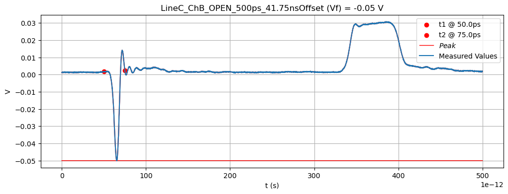
# Vf: LineA_ChB_OPEN_500ps_41.75nsOffset
WaveformPeakPlt(
LineA_ChB_OPEN_500ps_41,
x0=650,
x1=850,
total_time=500*10**(-12),
method='min',
mag=12,
unit='ps',
title='LineA_ChB_OPEN_500ps_41.75nsOffset (Vf)'
)
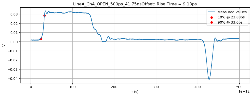
# Rise Time: LineA_ChA_OPEN_500ps_41.75nsOffset
WaveformRTimePlt(
LineA_ChA_OPEN_500ps_41,
x0=0, # Looks for rise time within Window Bounds [x0,x1]
x1=1000,
total_time=500*10**(-12),
fsv=0.0315,
mag=12,
unit='ps',
title='LineA_ChA_OPEN_500ps_41.75nsOffset'
)
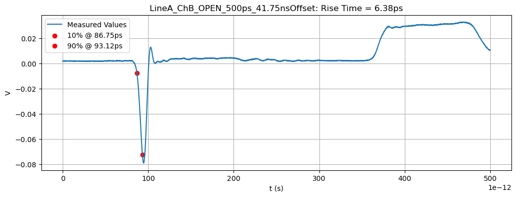
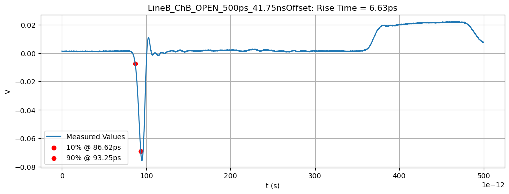
# Rise Time: LineA_ChB_OPEN_500ps_41.75nsOffset
WaveformRTimePlt(
LineA_ChB_OPEN_500ps_41,
x0=650,
x1=800,
total_time=500*10**(-12),
fsv=0.0792,
mag=12,
unit='ps',
title='LineA_ChB_OPEN_500ps_41.75nsOffset'
)
Analysis \(K_C\) and \(K_L\)
Given: \(d = 0.1 \text{m}\)
Measured:
\( \begin{eqnarray} & V_{b} &=& & 0.0315 \text{V} && t_{\text{rise}} &=& & 9.13 \text{ps} \\ & V_{f} &=& & -0.079 \text{V} && t_{\text{rise}} &=& & 6.38 \text{ps} \\ & v_0 &=& & 1.82 \cdot 10^8 \text{m/s} \\ & V_{\text{peak}} &=& & 0.25 \end{eqnarray}\)
Solve:
\(\begin{eqnarray} V_f &=& & \frac{K_C-K_L}{2v_0} \cdot d \cdot \frac{\partial V_{in}}{\partial t} \\ \\ V_f &=& & \frac{K_C-K_L}{2v_0} \cdot \frac{d}{t_{\text{rise}}} \cdot V_{\text{peak}}\\ \\ K_C-K_L &=& & 2 V_f v_0 \cdot \frac{t_{\text{rise}}}{d} \cdot \frac{1}{V_{\text{peak}}}\\ \\ K_C-K_L &=& & -0.0733 & (1)\\ \\ V_b &=& & \frac{K_C+K_L}{4}[V_{in}(t) - V_{in}(t-\frac{2d}{v_0})] && \rightarrow V_{\text{peak}} = [V_{in}(t) - V_{in}(t-\frac{2d}{v_0})] \\ \\ K_C+K_L &=& & \frac{4 V_b}{V_{\text{peak}}} \\ \\ K_C+K_L &=& & 0.504 & (2)\\ \end{eqnarray}\)
Summary \(K_C\) and \(K_L\)
Solving two equations with two unknowns. Thus \(K_C = 0.21522\) and \(K_L = 0.28879\).
Parameter |
Measured |
Given |
|---|---|---|
\(K_C\) |
0.21522 |
0.19890 |
\(K_L\) |
0.28879 |
0.26191 |
(3) Using the integration method, estimate the values of \(K_C\) and \(K_L\)#
# Define starting/ending points of input waveform
x10R,x90R = RiseTime( LineA_ChA_OPEN_500ps_41[0:1000] )
x90F,x10F = FallTime( LineA_ChA_OPEN_500ps_41[1000:1500] )

# Area Approximation: LineA_ChA_OPEN_500ps_41.75nsOffset
a = x90R
b = 1000+x90F
n = b-a
f = LineA_ChA_OPEN_500ps_41
offset = np.median(f[:100])
A = Waveform_Area(f,a,b,n,
    offset=offset,
    title='LineA_ChA_OPEN_500ps_41.75nsOffset'
)
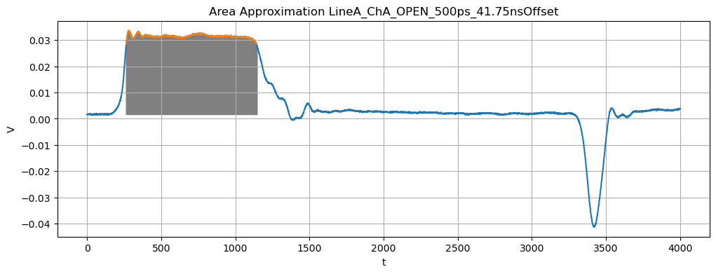
L = len(f)
x,res = np.linspace(0,500*10**(-12),L,endpoint=False,retstep=True)
A = A*res
print(f'Adjusted Area for Vb = {A}')
Adjusted Area for Vb = 3.2820425625000043e-12
# Area Approximation: LineA_ChB_OPEN_500ps_41.75nsOffset
a = 700
b = 800
n = b-a
f = LineA_ChB_OPEN_500ps_41
offset = 0
A = Waveform_Area(f,a,b,n,
    offset=offset,
    title='LineA_ChB_OPEN_500ps_41.75nsOffset'
)
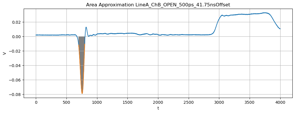
L = len(f)
x,res = np.linspace(0,500*10**(-12),L,endpoint=False,retstep=True)
A = A*res
print(f'Adjusted Area for Vf = {A}')
Adjusted Area for Vf = -6.17216125e-13
Measured:
\(\text{area}(V_b) = 3.2820 \cdot 10^{-12} \)
\(\text{area}(V_f) = -6.1721 \cdot 10^{-13} \)
Integration
\(\begin{eqnarray} \int_{0}^{\infty} V_f dt &=& \int_{0}^{\infty} [\frac{K_C-K_L}{2v_0} \cdot d \cdot \frac{d V_{in}}{dt}] dt && \rightarrow V_{\text{peak}} = V_{in}(t) - V_{in}(t-\frac{2d}{v_0})]\\ \\ &\approx& [\frac{K_C-K_L}{2v_0} \cdot d \cdot \frac{V_{\text{peak}}}{t_{\text{rise}}}] \int_{0}^{t_{\text{rise}}} dt \\ \\ \text{area}(V_f) &=& \frac{K_C-K_L}{2v_0} \cdot d \cdot V_{\text{peak}} \\ \\ K_C-K_L &=& \frac{2 v_0}{d \cdot V_{\text{peak}}} \text{area}(V_f) \\ \\ K_C-K_L &=& 0.0899 && (1)\\ \\ \int_{0}^{\infty} V_b dt &=& \int_{0}^{\infty} \frac{K_C-K_L}{4}[V_{in}(t) - V_{in}(t-\frac{2d}{v_0}]dt \\ \\ \text{area}(V_b) &=& \frac{K_C-K_L}{2v_0} \cdot V_{\text{peak}} * \frac{2d}{v_0} \\ \\ K_C+K_L &=& \frac{4 v_0}{2d \cdot V_{\text{peak}}} \text{area}(V_b) \\ \\ K_C+K_L &=& 0.4779 && (2)\\ \end{eqnarray}\)
Integration Summary \(K_C\) and \(K_L\)
Solving two equations with two unknowns. Thus \(K_C = 0.1940\) and \(K_L = 0.2839\).
Parameter |
Measured |
Given |
|---|---|---|
\(K_C\) |
0.1940 |
0.19220 |
\(K_L\) |
0.2839 |
0.28164 |
Estimation of \(C_{1G}, C_{2G}, C_{12}, L_{11}, L_{22}, L_{12} \)#
# Reflection Coefficient: LineA_Ch1Reflection_2ns_31.6nsOffset

np_arr = LineA_Ch1Reflection_2ns_31
total_time = 2*10**(-9)
method=None
mag=9
unit='V'
title='LineA_Ch1Reflection_2ns_31.6nsOffset'

# Figure
fig,ax = plt.subplots(figsize=(12,4))
L = len(np_arr)
x,res = np.linspace(0,total_time,L,endpoint=False,retstep=True)
Ures = res*10**mag

# Find V0 and V1
x0 = 1600
x1 = 1680
V0 = np_arr[x0][0]
V1 = np_arr[x1][0]

# Plot
ax.plot(x,np_arr,  # must be plotted in this order for Matplotlib
    color='red'
)
ax.scatter(x0*res,np_arr[x0],
    color='red',
    label=f'V0 @ {round(V0,4)}{unit}'
)
ax.scatter(x1*res,np_arr[x1],
    color='red',
    label=f'V1 @ {round(V1,4)}{unit}'
)
ax.plot(x,np.ones(L)*V0,
    color='red',
    linewidth=0.8
)
ax.plot(x,np.ones(L)*V1,
    color='red',
    linewidth=0.8
)
ax.plot(x,np_arr,
    label='Measured Values'
)

# Labels
ax.ticklabel_format(axis='x',style='sci', scilimits=(-mag,-mag))
ax.set_title(f'{title}: Reflection Coeff = {round((V1-V0)/V0,4)}')
ax.set_xlabel('t (s)')
ax.set_ylabel('V')
plt.grid(True)
plt.legend();
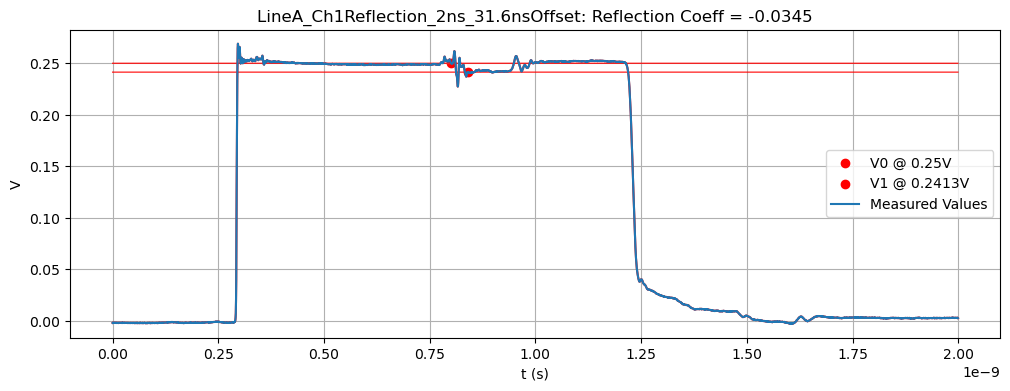
Unknown Parameters Analysis
Given:
\(\begin{eqnarray} C_{1G} && &=& && C_{2G} \\ L_{11} && &=& && L_{22} \\ K_C && &=& && 0.1940 \\ K_L && &=& && 0.2839 \\ v_0 && &=& && 1.82 \cdot 10^8 \text{m/s} \\ \Gamma && &=& && -0.0345 \end{eqnarray}\)
Solve:
\(\begin{eqnarray} C_1 && &=& && C_{1G} + C_{12} &=& && C_2 \\ \\ Z_{01} && &=& && \sqrt{\frac{L_{11}}{C_1}} &=& && \sqrt{\frac{L_{11}}{C_{1G}+C_{12}}} &=& && Z_{02} \\ v_1 && &=& && \frac{1}{\sqrt{L_{11}C_1}} &=& && \frac{1}{\sqrt{L_{11}(C_{1G}+C_{12})}} &=& && v_2 \\ K_C && &=& &&\frac{C_{12}}{C_{1G}+C_{12}} \\ \\ K_L && &=& &&\frac{L_{12}}{L_{11}} \end{eqnarray}\)
Calculations;
\(\begin{eqnarray} \Gamma && &=& && -0.0345 &=& && \frac{Z_{01}-Z_0}{Z_{01}+Z_0} \\ \\ && && && -0.0345 &=& && \frac{Z_{01}-50}{Z_{01}+50} \\ \\ && && && Z_{01} &=& && 46.67 \\ \\ 46.67 && &=& && \sqrt{\frac{L_{11}}{C_1}} &=& && \sqrt{\frac{L_{11}}{C_{1G}+C_{12}}} && (1) \\ 1.82\cdot 10^8 && &=& && \frac{1}{\sqrt{L_{11}C_1}} &=& && \frac{1}{\sqrt{L_{11}(C_{1G}+C_{12})}} && (2) \\ 0.1940 && &=& &&\frac{C_{12}}{C_{1G}+C_{12}} && && && (3)\\ \\ 0.2839 && &=& &&\frac{L_{12}}{L_{11}} && && && (4) \end{eqnarray}\)
C1G,C12,L11,L12,KC,KL,v0,Gamma = sp.symbols('C1G,C12,L11,L12,KC,KL,v0,Gamma')
system = sp.Matrix([
    [sp.sqrt(L11/(C1G+C12))-46.67],
    [1/sp.sqrt(L11*(C1G+C12))-1.82*10**8],
    [(C12)/(C1G+C12) - 0.1940],
    [(L12)/(L11) - 0.2939]
])
eq = sp.solve(system)
eq
[{C12: -2.28398128548118e-11,
  C1G: -9.48911812421562e-11,
  L11: -2.56428571428571e-7,
  L12: -7.53643571428571e-8},
 {C12: 2.28398128548118e-11,
  C1G: 9.48911812421562e-11,
  L11: 2.56428571428571e-7,
  L12: 7.53643571428571e-8}]
Unknown Parameters Summary
Solving four equations with four unknowns. The reflection of the coupled TL is necessary to calculate the reflection coefficient. Once we find this, we can find the individual characteristic impedance \(Z_{01}\). Find the self-capacitance (\(C_{1G}=C_{2G}\)), mutual capacitance (\(C_{12}\)), self-inductance(\(L_{11}, L_{22}\)), and mutual inductance(\(L_{12}\)) in the table.
Parameter |
units |
Measured |
Given |
|---|---|---|---|
\(v_0\) |
m/s |
\(1.82\) \(\cdot\) \(10^8\) |
\(1.71\) \(\cdot\) \(10^8\) |
\(K_C\) (method 1) |
\(0.2152\) |
\(0.19890\) |
|
\(K_L\) (method 1) |
\(0.2888\) |
\(0.26191\) |
|
\(K_C\) (integration method) |
\(0.1940\) |
\(0.19220\) |
|
\(K_L\) (integration method) |
\(0.2839\) |
\(0.28164\) |
|
\(Z_{01}\) |
ohms |
\(46.67\) |
\(45.97\) |
\(C_{12}\) |
pF |
\(22.83\) |
\(24.50\) |
\(C_{1G} = C_{2G}\) |
pF |
\(94.89\) |
\(102.77\) |
\(L_{11} = L_{22}\) |
nH |
\(256.43\) |
\(268.80\) |
\(L_{12}\) |
nH |
\(61.26\) |
\(75.71\) |
Coupled Lines
Coupled Lines |
A |
B |
C |
|---|---|---|---|
Coupled length d (cm) |
10 |
10 |
5 |
Line separation s (mm) |
0.5 |
1 |
0.5 |
Line B#
(1) Obtain the signal speed \(v_0\) on the TL using \(V_b\) waveform#
Assume the waveform is a square wave
# Signal Duration: LineB_ChA_OPEN_500ps_41nsOffset
#
fig,ax = plt.subplots(figsize=(12,4))
L = len(LineB_ChA_OPEN_500ps_41)
total_time = 500*10**(-12)
mag = 12
unit='ps'
x,res = np.linspace(0,total_time,L,endpoint=False,retstep=True)
Ures = res*10**mag

# Define starting/ending points of input waveform
x10R,x90R = RiseTime( LineB_ChA_OPEN_500ps_41[0:500] )
x90F,x10F = FallTime( LineB_ChA_OPEN_500ps_41[900:1500] )
x0 = x90R
x1 = 900+x90F

# Plot
ax.plot(x,LineB_ChA_OPEN_500ps_41,
    label='Measured Values'
)
ax.scatter(x0*res,LineB_ChA_OPEN_500ps_41[x0],
    color='red',
    label=f't1 @ {round(x0*Ures,2)}{unit}'
)
ax.scatter(x1*res,LineB_ChA_OPEN_500ps_41[x1],
    color='red',
    label=f't2 @ {round(x1*Ures,2)}{unit}'
)

# Labels
rt = RoundNonZeroDecimal((x1*Ures)-(x0*Ures),2)
ax.ticklabel_format(axis='x',style='sci', scilimits=(-mag,-mag))
ax.set_title(f'LineB_ChA_OPEN_500ps_41nsOffset: Signal Duration = {rt}{unit}')
ax.set_xlabel('t (s)')
ax.set_ylabel('V')
plt.grid(True)
plt.legend();
Given:
\(\begin{eqnarray} d &=& L = 0.10 \text{m} \end{eqnarray}\)
Measured:
\(\begin{eqnarray} t &=& 111.13 \text{ps} \end{eqnarray}\)
Solve:
\(\begin{eqnarray} \Delta T &=& \frac{2L}{v} \\ v &=& \frac{2L}{\Delta T} \\ v &=& \frac{2(0.10)}{111.13 \cdot 10^{-12}} \\ \\ &=& 1.7997 \cdot 10^8 \text{m/s} \end{eqnarray}\)
Signal Speed Summary#
Measured signal speed \(v_0\) on the TL using \(V_b\) waveform is \(1.7997 \cdot 10^8\) m/s.
(2) Using the peak values of \(V_b\) and \(V_f\), estimate \(K_C\) and \(K_L\)#
\([V_{in}(t) - V_{in}(t-\frac{2d}{v_0})] \rightarrow V_{\text{peak}}\)
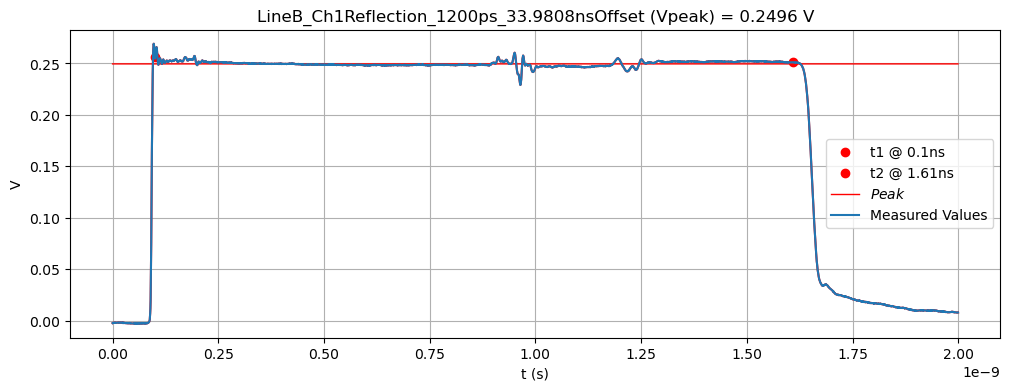
# Vpeak: LineB_Ch1Reflection_1200ps_33.9808nsOffset
WaveformPeakPlt(
LineB_Ch1Reflection_1200ps_33,
x0=200,
x1=3220,
total_time=2*10**(-9),
mag=9,
unit='ns',
title='LineB_Ch1Reflection_1200ps_33.9808nsOffset (Vpeak)'
)
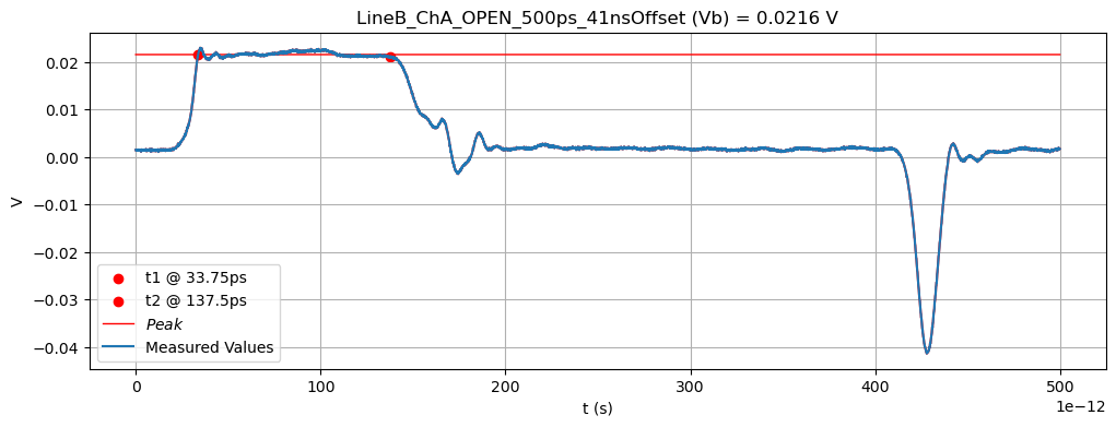
# Vb: LineB_ChA_OPEN_500ps_41nsOffset
WaveformPeakPlt(
LineB_ChA_OPEN_500ps_41,
x0=270,
x1=1100,
total_time=500*10**(-12),
mag=12,
unit='ps',
title='LineB_ChA_OPEN_500ps_41nsOffset (Vb)'
)
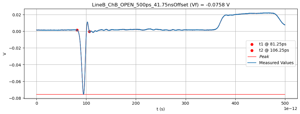
# Vf: LineB_ChB_OPEN_500ps_41.75nsOffset
WaveformPeakPlt(
LineB_ChB_OPEN_500ps_41,
x0=650,
x1=850,
total_time=500*10**(-12),
method='min',
mag=12,
unit='ps',
title='LineB_ChB_OPEN_500ps_41.75nsOffset (Vf)'
)
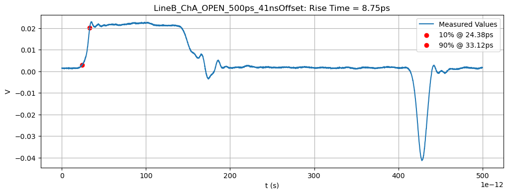
## Rise Time: LineB_ChA_OPEN_500ps_41nsOffset
WaveformRTimePlt(
    LineB_ChA_OPEN_500ps_41,
    x0=0,       # Looks for rise time within Window Bounds [x0,x1]
    x1=400,
    total_time=500*10**(-12),
    fsv=0.0315,
    mag=12,
    unit='ps',
    title='LineB_ChA_OPEN_500ps_41nsOffset'
)

# Fall Time: LineB_ChB_OPEN_500ps_41.75nsOffset
WaveformRTimePlt(
    LineB_ChB_OPEN_500ps_41,
    x0=500,
    x1=750,
    total_time=500*10**(-12),
    fsv=0.0758,
    mag=12,
    unit='ps',
    title='LineB_ChB_OPEN_500ps_41.75nsOffset'
)
Analysis \(K_C\) and \(K_L\)
Given:
\(\begin{eqnarray} d = 0.10 \text{m} \end{eqnarray}\)
Measured:
\( \begin{eqnarray} & V_{b} &=& & 0.0216 \text{V} && t_{\text{rise}} &=& & 8.75 \text{ps} \\ & V_{f} &=& & -0.0758 \text{V} && t_{\text{rise}} &=& & 6.63 \text{ps} \\ & v_0 &=& & 1.7997 \cdot 10^8 \text{m/s} \\ & V_{\text{peak}} &=& & 0.25 \end{eqnarray}\)
Solve:
\(\begin{eqnarray} K_C-K_L &=& & 2 V_f v_0 \cdot \frac{t_{\text{rise}}}{d} \cdot \frac{1}{V_{\text{peak}}}\\ \\ K_C+K_L &=& & \frac{4 V_b}{V_{\text{peak}}} \\ \\ K_C-K_L &=& & -0.00724 & (1)\\ \\ K_C+K_L &=& & 0.3456 & (2)\\ \end{eqnarray}\)
Summary \(K_C\) and \(K_L\)
Solving two equations with two unknowns. Thus \(K_C = 0.1692\) and \(K_L = 0.1764\).
Summary of \(\text{TL}_A\), \(\text{TL}_B\), \(\text{TL}_C\)#
Coupled Lines |
Coupled length d (m) |
Line separation s (m) |
\(V_b\) (V) |
\(V_f\) (V) |
b \(t_{\text{rise}}\) (ps) |
f \(t_{\text{rise}}\) (ps) |
\(K_C\) |
\(K_L\) |
|---|---|---|---|---|---|---|---|---|
A |
\(0.10\) |
\(0.0005\) |
\(0.2888\) |
\(0.0315\) |
\(9.13\) |
\(6.38\) |
\(0.2152\) |
\(0.2888\) |
B |
\(0.10\) |
\(0.0010\) |
\(0.1764\) |
\(0.0216\) |
\(8.75\) |
\(6.63\) |
\(0.1692\) |
\(0.1764\) |
C |
\(0.05\) |
\(0.0005\) |
\(0.0312\) |
\(0.0312\) |
\(8.75\) |
\(5.00\) |
\(0.2459\) |
\(0.2534\) |
The separation s affects the backwards coupled voltage \(V_b\) which is directly correlated to \(K_C\) and \(K_L\). As sepeation increases, the magnitude of \(V_b\) decreases. The coupled length d has no effect.
Line C#
(1) Obtain the signal speed \(v_0\) on the TL using \(V_b\) waveform#
Assume the waveform is a square wave
# Signal Duration: LineC_ChA_OPEN_500ps_41.75nsOffset
#
fig,ax = plt.subplots(figsize=(12,4))
L = len(LineC_ChA_OPEN_500ps_41)
total_time = 500*10**(-12)
mag = 12
unit='ps'
x,res = np.linspace(0,total_time,L,endpoint=False,retstep=True)
Ures = res*10**mag

# Define starting/ending points of input waveform
x10R,x90R = RiseTime( LineC_ChA_OPEN_500ps_41[0:500] )
x90F,x10F = FallTime( LineC_ChA_OPEN_500ps_41[500:1000] )
x0 = x90R
x1 = 500+x90F

# Plot
ax.plot(x,LineC_ChA_OPEN_500ps_41,
    label='Measured Values'
)
ax.scatter(x0*res,LineC_ChA_OPEN_500ps_41[x0],
    color='red',
    label=f't1 @ {round(x0*Ures,2)}{unit}'
)
ax.scatter(x1*res,LineC_ChA_OPEN_500ps_41[x1],
    color='red',
    label=f't2 @ {round(x1*Ures,2)}{unit}'
)

# Labels
rt = RoundNonZeroDecimal((x1*Ures)-(x0*Ures),2)
ax.ticklabel_format(axis='x',style='sci', scilimits=(-mag,-mag))
ax.set_title(f'LineC_ChA_OPEN_500ps_41.75nsOffset: Signal Duration = {rt}{unit}')
ax.set_xlabel('t (s)')
ax.set_ylabel('V')
plt.grid(True)
plt.legend();
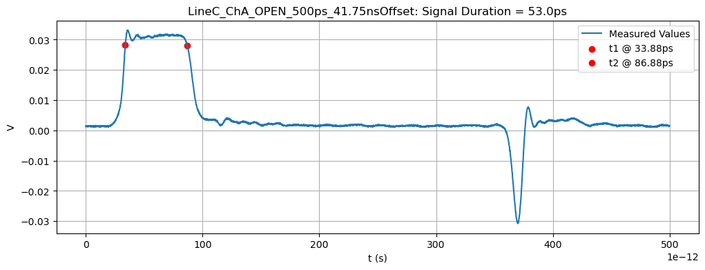
Given:
\(\begin{eqnarray} d &=& L = 0.05 \text{m} \end{eqnarray}\)
Measured:
\(\begin{eqnarray} t &=& 53 \text{ps} \end{eqnarray}\)
Solve:
\(\begin{eqnarray} \Delta T &=& \frac{2L}{v} \\ v &=& \frac{2L}{\Delta T} \\ v &=& \frac{2(0.05)}{53 \cdot 10^{-12}} \\ \\ &=& 1.8868 \cdot 10^8 \text{m/s} \end{eqnarray}\)
Signal Speed Summary#
Measured signal speed \(v_0\) on the TL using \(V_b\) waveform is \(1.8868 \cdot 10^8\) m/s.
(2) Using the peak values of \(V_b\) and \(V_f\), estimate \(K_C\) and \(K_L\)#
\([V_{in}(t) - V_{in}(t-\frac{2d}{v_0})] \rightarrow V_{\text{peak}}\)
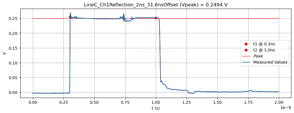
# Vpeak: LineC_Ch1Reflection_2.4ns_30.91nsOffset
WaveformPeakPlt(
LineC_Ch1Reflection_2ns_30,
x0=607,
x1=2000,
total_time=2*10**(-9),
mag=9,
unit='ns',
title='LineC_Ch1Reflection_2ns_31.6nsOffset (Vpeak)'
)
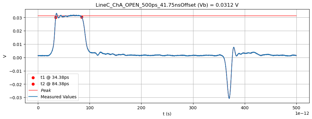
# Vb: LineC_ChA_OPEN_500ps_41.75nsOffset
WaveformPeakPlt(
LineC_ChA_OPEN_500ps_41,
x0=275,
x1=675,
total_time=500*10**(-12),
mag=12,
unit='ps',
title='LineC_ChA_OPEN_500ps_41.75nsOffset (Vb)'
)
# Vf: LineC_ChB_OPEN_500ps_41.75nsOffset
WaveformPeakPlt(
LineC_ChB_OPEN_500ps_41,
x0=400,
x1=600,
total_time=500*10**(-12),
method='min',
mag=12,
unit='ps',
title='LineC_ChB_OPEN_500ps_41.75nsOffset (Vf)'
)
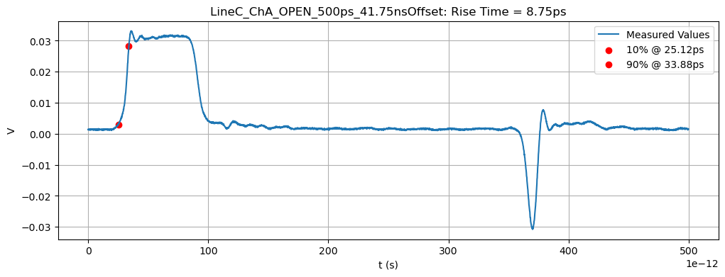
## Rise Time: LineC_ChA_OPEN_500ps_41.75nsOffset
WaveformRTimePlt(
LineC_ChA_OPEN_500ps_41,
x0=0, # Looks for rise time within Window Bounds [x0,x1]
x1=500,
total_time=500*10**(-12),
fsv=0.0315,
mag=12,
unit='ps',
title='LineC_ChA_OPEN_500ps_41.75nsOffset'
)
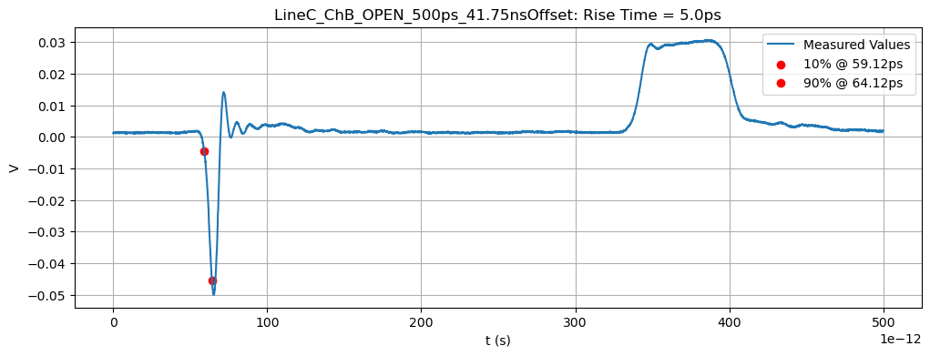
# Fall Time: LineC_ChB_OPEN_500ps_41.75nsOffset
WaveformRTimePlt(
LineC_ChB_OPEN_500ps_41,
x0=0,
x1=530,
total_time=500*10**(-12),
fsv=0.05,
mag=12,
unit='ps',
title='LineC_ChB_OPEN_500ps_41.75nsOffset'
)
Analysis \(K_C\) and \(K_L\)
Given: \(d = 0.05 \text{m}\)
Measured:
\( \begin{eqnarray} & V_{b} &=& & 0.0312 \text{V} && t_{\text{rise}} &=& & 8.75 \text{ps} \\ & V_{f} &=& & -0.05 \text{V} && t_{\text{rise}} &=& & 5.0 \text{ps} \\ & v_0 &=& & 1.8868 \cdot 10^8 \text{m/s} \\ & V_{\text{peak}} &=& & 0.25 \end{eqnarray}\)
Solve:
\(\begin{eqnarray} K_C-K_L &=& & 2 V_f v_0 \cdot \frac{t_{\text{rise}}}{d} \cdot \frac{1}{V_{\text{peak}}}\\ \\ K_C+K_L &=& & \frac{4 V_b}{V_{\text{peak}}} \\ \\ K_C-K_L &=& & -0.0075 & (1)\\ \\ K_C+K_L &=& & 0.4992 & (2)\\ \end{eqnarray}\)
Summary \(K_C\) and \(K_L\)
Solving two equations with two unknowns. Thus \(K_C = 0.2459\) and \(K_L = 0.2534\).
Tranmission Line Analysis#
Transmission Line A - already included#
Transmission Line B#
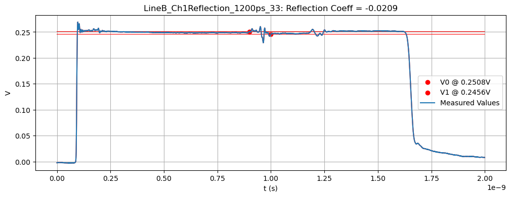
# Reflection Coefficient: LineB_Ch1Reflection_1200ps_33

np_arr = LineB_Ch1Reflection_1200ps_33
total_time = 2*10**(-9)
method=None
mag=9
unit='V'
title='LineB_Ch1Reflection_1200ps_33'

# Figure
fig,ax = plt.subplots(figsize=(12,4))
L = len(np_arr)
x,res = np.linspace(0,total_time,L,endpoint=False,retstep=True)
Ures = res*10**mag

# Find V0 and V1
x0 = 1800
x1 = 2000
V0 = np_arr[x0][0]
V1 = np_arr[x1][0]

# Plot
ax.plot(x,np_arr,  # must be plotted in this order for Matplotlib
    color='red'
)
ax.scatter(x0*res,np_arr[x0],
    color='red',
    label=f'V0 @ {round(V0,4)}{unit}'
)
ax.scatter(x1*res,np_arr[x1],
    color='red',
    label=f'V1 @ {round(V1,4)}{unit}'
)
ax.plot(x,np.ones(L)*V0,
    color='red',
    linewidth=0.8
)
ax.plot(x,np.ones(L)*V1,
    color='red',
    linewidth=0.8
)
ax.plot(x,np_arr,
    label='Measured Values'
)

# Labels
ax.ticklabel_format(axis='x',style='sci', scilimits=(-mag,-mag))
ax.set_title(f'{title}: Reflection Coeff = {round((V1-V0)/V0,4)}')
ax.set_xlabel('t (s)')
ax.set_ylabel('V')
plt.grid(True)
plt.legend();
Given:
\(\begin{eqnarray} C_{1G} &= C_{2G} \\ L_{11} &= L_{22} \\ K_C &= 0.1692 \\ K_L &= 0.1764 \\ v_0 &= 1.80 \cdot 10^8 \text{m/s} \\ \Gamma &= -0.0209 \end{eqnarray}\)
Solve:
\(\begin{eqnarray} C_1 && &=& && C_{1G} + C_{12} &=& && C_2 \\ \\ Z_{01} && &=& && \sqrt{\frac{L_{11}}{C_1}} &=& && \sqrt{\frac{L_{11}}{C_{1G}+C_{12}}} &=& && Z_{02} \\ v_1 && &=& && \frac{1}{\sqrt{L_{11}C_1}} &=& && \frac{1}{\sqrt{L_{11}(C_{1G}+C_{12})}} &=& && v_2 \\ K_C && &=& &&\frac{C_{12}}{C_{1G}+C_{12}} \\ \\ K_L && &=& &&\frac{L_{12}}{L_{11}} \end{eqnarray}\)
Calculations:
\(\begin{eqnarray} \Gamma && &=& && -0.0678 &=& && \frac{Z_{01}-Z_0}{Z_{01}+Z_0} \\ \\ && && && -0.0678 &=& && \frac{Z_{01}-50}{Z_{01}+50} \\ \\ && && && Z_{01} &=& && 46.67 \\ \\ 47.95 && &=& && \sqrt{\frac{L_{11}}{C_1}} &=& && \sqrt{\frac{L_{11}}{C_{1G}+C_{12}}} && (1) \\ 1.80\cdot 10^8 && &=& && \frac{1}{\sqrt{L_{11}C_1}} &=& && \frac{1}{\sqrt{L_{11}(C_{1G}+C_{12})}} && (2) \\ 0.1692 && &=& &&\frac{C_{12}}{C_{1G}+C_{12}} && && && (3)\\ \\ 0.1764 && &=& &&\frac{L_{12}}{L_{11}} && && && (4) \end{eqnarray}\)
C1G,C12,L11,L12,KC,KL,v0,Gamma = sp.symbols('C1G,C12,L11,L12,KC,KL,v0,Gamma')
system = sp.Matrix([
    [sp.sqrt(L11/(C1G+C12))-47.95],
    [1/sp.sqrt(L11*(C1G+C12))-1.80*10**8],
    [(C12)/(C1G+C12) - 0.1692],
    [(L12)/(L11) - 0.1764]
])
eq = sp.solve(system)
eq
[{C12: -1.96037539103233e-11,
  C1G: -9.62576758197196e-11,
  L11: -2.66388888888889e-7,
  L12: -4.69910000000000e-8},
 {C12: 1.96037539103233e-11,
  C1G: 9.62576758197196e-11,
  L11: 2.66388888888889e-7,
  L12: 4.69910000000000e-8}]
Transmission Line C#
# Reflection Coefficient: LineC_Ch1Reflection_2ns_30

np_arr = LineC_Ch1Reflection_2ns_30
total_time = 2*10**(-9)
method=None
mag=9
unit='V'
title='LineC_Ch1Reflection_2ns_30'

# Figure
fig,ax = plt.subplots(figsize=(12,4))
L = len(np_arr)
x,res = np.linspace(0,total_time,L,endpoint=False,retstep=True)
Ures = res*10**mag

# Find V0 and V1
x0 = 1410
x1 = 1520
V0 = np_arr[x0][0]
V1 = np_arr[x1][0]

# Plot
ax.plot(x,np_arr,  # must be plotted in this order for Matplotlib
    color='red'
)
ax.scatter(x0*res,np_arr[x0],
    color='red',
    label=f'V0 @ {round(V0,4)}{unit}'
)
ax.scatter(x1*res,np_arr[x1],
    color='red',
    label=f'V1 @ {round(V1,4)}{unit}'
)
ax.plot(x,np.ones(L)*V0,
    color='red',
    linewidth=0.8
)
ax.plot(x,np.ones(L)*V1,
    color='red',
    linewidth=0.8
)
ax.plot(x,np_arr,
    label='Measured Values'
)

# Labels
ax.ticklabel_format(axis='x',style='sci', scilimits=(-mag,-mag))
ax.set_title(f'{title}: Reflection Coeff = {round((V1-V0)/V0,4)}')
ax.set_xlabel('t (s)')
ax.set_ylabel('V')
plt.grid(True)
plt.legend();
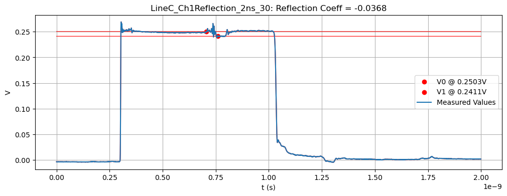
Given:
\(\begin{eqnarray} C_{1G} &= C_{2G} \\ L_{11} &= L_{22} \\ K_C &= 0.2459 \\ K_L &= 0.2534 \\ v_0 &= 1.89 \cdot 10^8 \text{m/s} \\ \Gamma &= -0.0368 \end{eqnarray}\)
Solve:
\(\begin{eqnarray} C_1 && &=& && C_{1G} + C_{12} &=& && C_2 \\ \\ Z_{01} && &=& && \sqrt{\frac{L_{11}}{C_1}} &=& && \sqrt{\frac{L_{11}}{C_{1G}+C_{12}}} &=& && Z_{02} \\ v_1 && &=& && \frac{1}{\sqrt{L_{11}C_1}} &=& && \frac{1}{\sqrt{L_{11}(C_{1G}+C_{12})}} &=& && v_2 \\ K_C && &=& &&\frac{C_{12}}{C_{1G}+C_{12}} \\ \\ K_L && &=& &&\frac{L_{12}}{L_{11}} \end{eqnarray}\)
Calculations;
\(\begin{eqnarray} \Gamma && &=& && -0.0368 &=& && \frac{Z_{01}-Z_0}{Z_{01}+Z_0} \\ \\ && && && -0.0368 &=& && \frac{Z_{01}-50}{Z_{01}+50} \\ \\ && && && Z_{01} &=& && 46.45 \\ \\ 46.45 && &=& && \sqrt{\frac{L_{11}}{C_1}} &=& && \sqrt{\frac{L_{11}}{C_{1G}+C_{12}}} && (1) \\ 1.89\cdot 10^8 && &=& && \frac{1}{\sqrt{L_{11}C_1}} &=& && \frac{1}{\sqrt{L_{11}(C_{1G}+C_{12})}} && (2) \\ 0.2459 && &=& &&\frac{C_{12}}{C_{1G}+C_{12}} && && && (3)\\ \\ 0.2534 && &=& &&\frac{L_{12}}{L_{11}} && && && (4) \end{eqnarray}\)
C1G,C12,L11,L12,KC,KL,v0,Gamma = sp.symbols('C1G,C12,L11,L12,KC,KL,v0,Gamma')
system = sp.Matrix([
    [sp.sqrt(L11/(C1G+C12))-46.45],
    [1/sp.sqrt(L11*(C1G+C12))-1.89*10**8],
    [(C12)/(C1G+C12) - 0.2459],
    [(L12)/(L11) - 0.2534]
])
eq = sp.solve(system)
eq
[{C12: -2.80098643930721e-11,
  C1G: -8.58976768556962e-11,
  L11: -2.45767195767196e-7,
  L12: -6.22774074074074e-8},
 {C12: 2.80098643930721e-11,
  C1G: 8.58976768556962e-11,
  L11: 2.45767195767196e-7,
  L12: 6.22774074074074e-8}]
Parameter Summary#
Transmission Line A |
units |
Measured |
Given |
|---|---|---|---|
\(v_0\) |
m/s |
\(1.82\) \(\cdot\) \(10^8\) |
\(1.71\) \(\cdot\) \(10^8\) |
\(K_C\) (method 1) |
\(0.2152\) |
\(0.19890\) |
|
\(K_L\) (method 1) |
\(0.2888\) |
\(0.26191\) |
|
\(K_C\) (integration method) |
\(0.1940\) |
\(0.19220\) |
|
\(K_L\) (integration method) |
\(0.2839\) |
\(0.28164\) |
|
\(Z_{01}\) |
ohms |
\(46.67\) |
\(45.97\) |
\(C_{12}\) |
pF |
\(22.83\) |
\(24.50\) |
\(C_{1G} = C_{2G}\) |
pF |
\(94.89\) |
\(102.77\) |
\(L_{11} = L_{22}\) |
nH |
\(256.43\) |
\(268.80\) |
\(L_{12}\) |
nH |
\(61.26\) |
\(75.71\) |
Transmission Line B |
units |
Measured |
|---|---|---|
\(v_0\) |
m/s |
\(1.80\) \(\cdot\) \(10^8\) |
\(K_C\) (method 1) |
\(0.2152\) |
|
\(K_L\) (method 1) |
\(0.2888\) |
|
\(Z_{01}\) |
ohms |
\(46.67\) |
\(C_{12}\) |
pF |
\(19.60\) |
\(C_{1G} = C_{2G}\) |
pF |
\(96.26\) |
\(L_{11} = L_{22}\) |
nH |
\(266.38\) |
\(L_{12}\) |
nH |
\(46.99\) |
Transmission Line C |
units |
Measured |
|---|---|---|
\(v_0\) |
m/s |
\(1.89\) \(\cdot\) \(10^8\) |
\(K_C\) (method 1) |
\(0.2459\) |
|
\(K_L\) (method 1) |
\(0.2534\) |
|
\(Z_{01}\) |
ohms |
\(47.95\) |
\(C_{12}\) |
pF |
\(28.01\) |
\(C_{1G} = C_{2G}\) |
pF |
\(85.90\) |
\(L_{11} = L_{22}\) |
nH |
\(245.77\) |
\(L_{12}\) |
nH |
\(62.28\) |
Questions#
1. Changes in coupled noise polarity due to load type#
Data |
Coupling |
Short |
Open |
||
|---|---|---|---|---|---|
rising edge |
falling edge |
rising edge |
falling edge |
||
LineA_ChA |
backwards |
pos |
neg |
pos |
pos |
LineA_ChB |
forwards |
neg |
pos |
neg |
neg |
LineB_ChA |
backwards |
pos |
neg |
pos |
pos |
LineB_ChB |
forwards |
neg |
pos |
neg |
neg |
LineC_ChA |
backwards |
pos |
neg |
pos |
pos |
LineC_ChB |
forwards |
neg |
pos |
neg |
neg |
Backward coupled noise follows the same polarity of the input square wave for SHORT termination.
Backward coupled noise remains positive regardless of the input square wave slope for OPEN termination.
Forward coupled noise follows the opposite polarity of the input square wave for SHORT termination.
Forward coupled noise remains negative regardless of the input square wave slope for OPEN termination.
2. Show \(K_C\) and \(K_L\) are dependent on the separation \(s\) and independent of length \(d\).#
Original \(K_C\) and \(K_L\) were calculated with Line A of distance \(d = 0.1\)m and separation \(s = 0.0005\)m.
Repeat ‘Analysis and Estimation of \(K_C\) and \(K_L\)’ with Line B of distance \(d = 0.10\)m and separation \(s = 0.001\)m.
Repeat ‘Analysis and Estimation of \(K_C\) and \(K_L\)’ with Line C of distance \(d = 0.05\)m and separation \(s = 0.0005\)m.
Coupled noise waveforms#
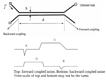
(a) Short load type is attached at Port 2 (thru port).
(b) Explain the waveforms A and B are not the same.
Forward coupled noise has the following characteristics:
magnitude of the forward coupled noise is linearly proportional to the coupled length
pulse width is related to the rise-time
rise-time (positive slope) of the input signal will create a negative pulse and fall-time will create a positive pulse
exists for microstrip but not stripline TLs
Given the coupled TL is lossy, the magnitude of forward coupled waveform A is less affected than the backward coupled waveform B since the signal has to travel further for B.
(c) Explain the waveforms C and D are not the same.
Backward coupled noise has the following characteristics:
pulse width is related to the length of the coupled section
magnitude of the backward coupled noise is not proportional to the coupled length
rise-time (positive slope) of the input signal will create a positive pulse and fall-time will create a negative pulse
exists for miscrostrip and stipline TLs
The observed signals for backward coupled noise don’t arrive at the same time since the travel distance is not the same. These are possible differences in C and D.
Conclusion#
Measured signal speed and forward/backward peak voltages
Found coupling coefficients (\(K_C\) and \(K_L\)) in transmission lines A,B,C.
Observed coupled noise is dependent to separation distance and independent to coupling length.
Observed polarity relationship of forward/backward waveforms to open and short loads.
Calculated lumped element model for coupled transmission lines.