Time-Domain Analysis#

Due: January 22, 2020

Author: Kevin Egedy

Objectives#

I. Measurement of the verification devices:

Match the waveforms to the three loads: short, open and match, and find the reflection coefficient of each.

II. Unmatached TL:

Identify the location of the impedance discontinuity.
Evaluate the values of characteristic impedance of each TL section of the board. Main one is 100 ohm section.
Estimate the dielectric constant of 100 ohm TL.

III. Unknown loads:

Based on the expected responses and the time-domain responses of complex loads, estimate the characteristics (capacitive, resistive, inductive, or combination of these?) and values of these loads(include the analysis process)

IV. Small Inductance

From the measured decay constant, using the relation \(L = R_st\), compute the inductance of the DUT. If the decay time is too short, skip this part.
From the measured total area under a response curve, compute the inductance of the DUT.

# Libraries
#
import pandas as pd
import numpy as np
import matplotlib.pyplot as plt
import matplotlib.patches as pch
%matplotlib inline
from IPython.core.interactiveshell import InteractiveShell
InteractiveShell.ast_node_interactivity = "all"

files = [
    'calib_matched_garman',
    'calib_open_garman',
    'calib_short_garman',
    'Part1-PCBduroid',
    'Part1-unknown1',
    'Part1-unknown2',
    'Part1-unknown3_1ns',
    'Part1-unknown3_260ps',
    'Part2-board2_280ps',
    'Part2-calib_ch2_Thu'
]

%%capture
# Read .xlsx files and convert them into .csv
#
for filename in files:
    df = pd.read_excel(f'data/{filename}.xlsx',header=None,nrows=1)
    with open(f'data/csv/{filename}.csv','w+') as f0: f0.write(df.T.to_csv(index=False,header=None));

# Read .csv files in lab01/data/csv
#
calib_matched_garman = pd.read_csv('data/csv/calib_matched_garman.csv',header=None).to_numpy()
calib_open_garman    = pd.read_csv('data/csv/calib_open_garman.csv',header=None).to_numpy()
calib_short_garman   = pd.read_csv('data/csv/calib_short_garman.csv',header=None).to_numpy()
Part1_PCBduroid      = pd.read_csv('data/csv/Part1-PCBduroid.csv',header=None).to_numpy()
Part1_unknown1       = pd.read_csv('data/csv/Part1-unknown1.csv',header=None).to_numpy()
Part1_unknown2       = pd.read_csv('data/csv/Part1-unknown2.csv',header=None).to_numpy()
Part1_unknown3_1ns   = pd.read_csv('data/csv/Part1-unknown3_1ns.csv',header=None).to_numpy()
Part1_unknown3_260ps = pd.read_csv('data/csv/Part1-unknown3_260ps.csv',header=None).to_numpy()
Part2_board2_280ps   = pd.read_csv('data/csv/Part2-board2_280ps.csv',header=None).to_numpy()
Part2_calib_ch2_Thu  = pd.read_csv('data/csv/Part2-calib_ch2_Thu.csv',header=None).to_numpy()

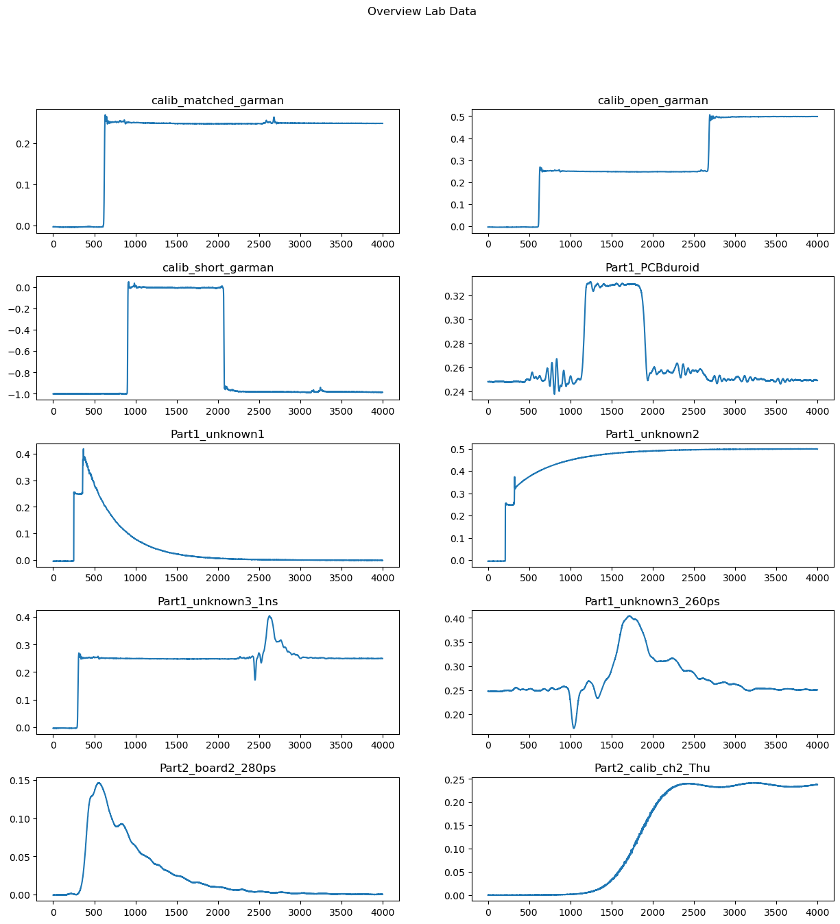
# Plot Overview
#   Number of points: 4000pts
#   Total Time: 200ns
#   Resolution: 0.05 ns/pt
#
fig,axs = plt.subplots(5,2,figsize=(15,15))
plt.subplots_adjust(hspace=0.35)
plt.subplots_adjust(wspace=0.20)

axs[0,0].plot(calib_matched_garman)
axs[0,1].plot(calib_open_garman)
axs[1,0].plot(calib_short_garman)
axs[1,1].plot(Part1_PCBduroid)
axs[2,0].plot(Part1_unknown1)
axs[2,1].plot(Part1_unknown2)
axs[3,0].plot(Part1_unknown3_1ns)
axs[3,1].plot(Part1_unknown3_260ps)
axs[4,0].plot(Part2_board2_280ps)
axs[4,1].plot(Part2_calib_ch2_Thu)

axs[0,0].set_title('calib_matched_garman')
axs[0,1].set_title('calib_open_garman')
axs[1,0].set_title('calib_short_garman')
axs[1,1].set_title('Part1_PCBduroid')
axs[2,0].set_title('Part1_unknown1')
axs[2,1].set_title('Part1_unknown2')
axs[3,0].set_title('Part1_unknown3_1ns')
axs[3,1].set_title('Part1_unknown3_260ps')
axs[4,0].set_title('Part2_board2_280ps')
axs[4,1].set_title('Part2_calib_ch2_Thu')
plt.suptitle('Overview Lab Data');

../../_images/time-domain-response_7_0.png

Constants#

Permittivity of free-space \(= \epsilon_0 = 8.854 \cdot 10^{-12} F/m\)
Permeability of free-space \(= \mu_0 = 4\pi \cdot 10^{-7} H/m\)
Impedance of free-space \(= \eta_0 = 120\pi = 376.7\Omega\)
Velocity of light in free-space \(= c = 2.998 \cdot 10^8 m/s\)

Helpful Equations#

\(\begin{align} \Gamma_L &= \frac{V^-}{V^+} = \frac{Z_L-Z_0}{Z_L+Z_0} \end{align}\)

\(\Delta T = \frac{2L}{v} \) where \(L\) = length, \(T\) = time delay and \(v\) = velocity

\(\tau\) is time to reach \(63.2\%\) of its final value in an increasing system and \(36.8\%\) is a decreasing system.

Characteristic Impedance of TL: TEM

\(\begin{eqnarray} z_0 &=& \sqrt{\frac{L}{C}} &=& \sqrt{\frac{\mu}{\epsilon}}\\ v &=& \frac{1}{\sqrt{LC}} &=& \frac{1}{\sqrt{\mu \epsilon}} &=& \frac{c_0}{\sqrt{\epsilon_r}} \end{eqnarray}\)

Microstrip Effective Permitivity \(\epsilon_{eff}\)

\(\begin{eqnarray} \epsilon_{eff} &=& \frac{\epsilon_r+1}{2} + \frac{\epsilon_r-1}{2} (\frac{1}{\sqrt{1+12d/W}}) \end{eqnarray}\)

TDS8200 setup#

Instructions

Read the attached file for instruction
Only Ch 1 must be set to TDR (red LED ON). Under MEASURE
The red LED of Ch 2 must be OFF
Time scale and number of points: These can be found from Setup->Hori

(1) Measurement of the Verification Devices#

Instructions

Attach SHORT to the end of cable and obtain the reflection from it
- Save data into PC
Attach the matched load and obtain the reflection from it
Do not attach any devices and measure the reflection (OPEN)

Questions

Find the reflection coefficient from the open, short and matched waveforms

# Measured Values: Part1_unknown1
#
fig,axs = plt.subplots(3,1,figsize=(12,12))
plt.subplots_adjust(hspace=0.35)
x = np.linspace(0,10*10**(-9),len(calib_short_garman))

# Plot
axs[0].plot(x,calib_short_garman,label='Short')
axs[1].plot(x,calib_matched_garman,label='Matched')
axs[2].plot(x,calib_open_garman,label='Open')

# Labels
axs[0].set_title('Short')
axs[1].set_title('Matched')
axs[2].set_title('Open')

axs[0].set_ylabel('V')
axs[1].set_ylabel('V')
axs[2].set_ylabel('V')

axs[0].set_xlabel('t (s)')
axs[1].set_xlabel('t (s)')
axs[2].set_xlabel('t (s)')

axs[0].ticklabel_format(axis='x',style='sci', scilimits=(-9,-9))
axs[1].ticklabel_format(axis='x',style='sci', scilimits=(-9,-9))
axs[2].ticklabel_format(axis='x',style='sci', scilimits=(-9,-9))

axs[0].grid(True)
axs[1].grid(True)
axs[2].grid(True)

plt.suptitle('Calibration Measured Values');

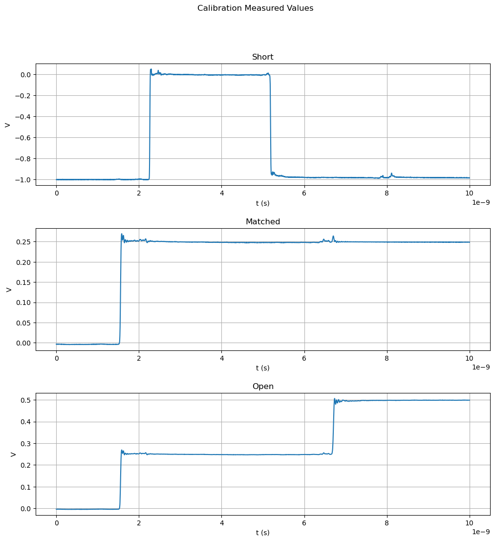
../../_images/time-domain-response_12_0.png

Reflection Coefficients

\(\begin{align} \Gamma_L &= \frac{V^-}{V^+} \end{align}\)

\(\begin{align} &V^+ =& -1.0V && V^- &=& 1.0V && \rightarrow \Gamma_{short} &=-1 \\ &V^+ =& 0.25V && V^- &=& 0V && \rightarrow \Gamma_{match} &= 0 \\ &V^+ =& 0.25V && V^- &=& 0.25V && \rightarrow \Gamma_{open} &= 1 \end{align}\)

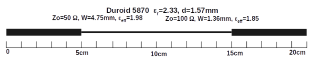
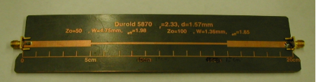
(2) Unmatched Transmission Line#

Instructions

Connect a test board with the matched impedance (terminated with \(Z_L=50\)) and measure the reflection from it.
- Save data into PC.

Questions

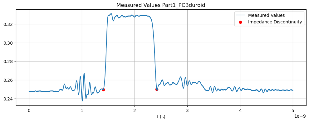
Identify the location of the impedance discontinuity and values of the characteristic impedance
From the measured time delay, estimate the dielectric constant and characteristic impedance of each TL section of the board

# Measured Values: Part1_unknown1
#
fig,ax = plt.subplots(figsize=(12,4))
x = np.linspace(0,5*10**(-9),len(Part1_PCBduroid))
res = 1.25*10**(-12) # 1.25 ps

# Impedance Discontinuity
x1 = 1125
x2 = 1935

# Plot
ax.plot(x,Part1_PCBduroid,label='Measured Values')
ax.scatter(x1*res,Part1_PCBduroid[x1],color='red')
ax.scatter(x2*res,Part1_PCBduroid[x2],color='red',label='Impedance Discontinuity')

# Labels
ax.ticklabel_format(axis='x',style='sci', scilimits=(-9,-9))
ax.set_title('Measured Values Part1_PCBduroid')
ax.set_xlabel('t (s)')
plt.legend()
plt.grid(True);

../../_images/time-domain-response_16_0.png

Find velocity:

\(\begin{eqnarray} \Delta T &=& \frac{2L}{v} \\ v &=& \frac{2L}{\Delta T} \end{eqnarray}\)

Use velocity to find \(\epsilon_{r}\)

\(\begin{eqnarray} v &=& \frac{c_0}{\sqrt{\epsilon_r}} \\ \sqrt{\epsilon_r} &=& \frac{c_0}{v} \\ \epsilon_r &=& (\frac{c_0}{v})^2 \end{eqnarray}\)

# Calculate Dielectric Constant

# speed of light
c0= 2.998*10**(8)

# length
L = 0.10

# time
t = x2*res - x1*res

# velocity
v = 2*L/t

# dielectric constant
eps = (c0/v)**2

print(f'Dielectric constant: measured = {round(eps,4)} F/m, given: 2.33 F/m') # 100 Ohm TL Section

Dielectric constant: measured = 2.3035 F/m, given: 2.33 F/m

Check by solving dielectric effective (microstrip)

\(\begin{eqnarray} \epsilon_{eff} &=& \frac{\epsilon_r+1}{2} + \frac{\epsilon_r-1}{2} (\frac{1}{\sqrt{1+12d/W}}) \end{eqnarray}\)

# Check Measured Values
#
def eps_eff(Er,d,W):
    return (Er+1)/2+(Er-1)*(1/np.sqrt(1+12*d/W))/2

Er = 2.3035
d = 0.00157
W = 0.00136
print(f'Dielectric effective: measured = {round(eps_eff(Er,d,W),4)} F/m, \
given: 1.85 F/m')

Dielectric effective: measured = 1.8209 F/m, given: 1.85 F/m

Use reflection coefficient to find characteristic impedance \(Z_0\)

\(\begin{eqnarray} \Gamma_{t_1} &=& \frac{V^-}{V^+} &=& \frac{(0.33-0.25)}{0.25} &=& 0.32 \\ \Gamma_{t_2} &=& \frac{V^-}{V^+} &=& \frac{(0.33-0.25)}{0.25} &=& -0.32 \end{eqnarray}\)

Given test board is terminated with 50 Ohms - work from sink to source.

\(\begin{align} \Gamma_L &= \frac{Z_L-Z_0}{Z_L+Z_0} \\ \Gamma_{t_2} &= -0.32 &=& \frac{50-Z_0}{50+Z_0} && \rightarrow Z_L = 50, Z_0 = 97.06 \\ \Gamma_{t_1} &= 0.32 &=& \frac{97.06-Z_0}{97.06+Z_0} && \rightarrow Z_L = 97.06, Z_0 = 50 \end{align}\)

print(f'TL Section 1 Z0: measured = 50.00 Ohms, given 50 Ohms')
print(f'TL Section 2 Z0: measured = 97.06 Ohms, given 100 Ohms')
print(f'TL Section 3 Z0: measured = 50.00 Ohms, given 50 Ohms')

TL Section 1 Z0: measured = 50.00 Ohms, given 50 Ohms
TL Section 2 Z0: measured = 97.06 Ohms, given 100 Ohms
TL Section 3 Z0: measured = 50.00 Ohms, given 50 Ohms

Unmatched Transmission Line Summary

	Section 1	Section 2	Section 3
dielectric constant (F/m)	NA	2.3035	NA
characteristic impedance (Ohms)	50.0	97.06	50.0

(3) Unknown Loads#

Instructions

Measure three unknown loads and save results.

Questions

Using the analytical model, estimate the characteristics (capacitive, resistive, inductive, or combination of these?) and values of these loads.
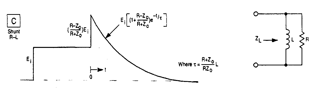
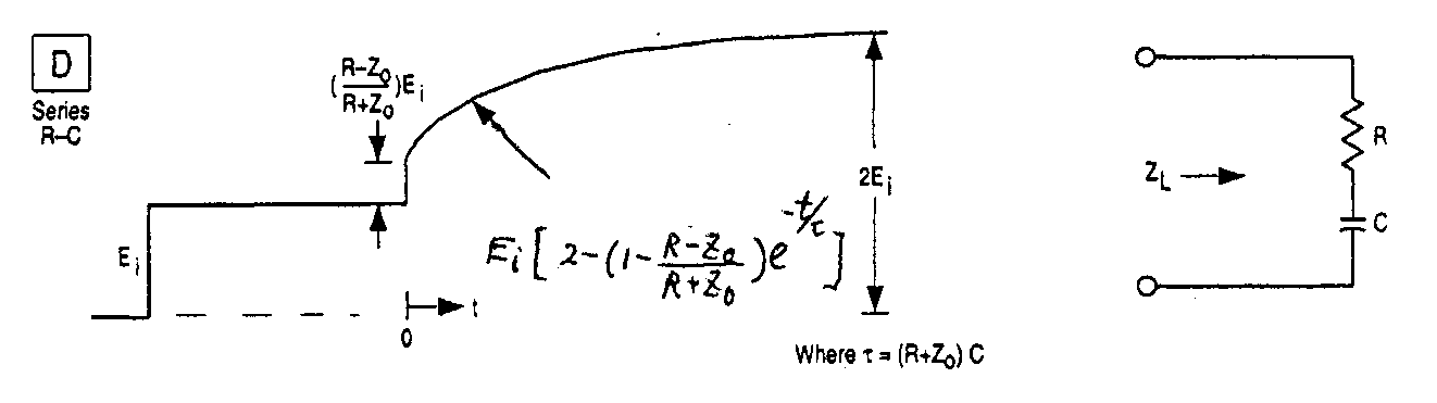
See the expected responses and the time-domain responses of complex loads.

Part1_unknown1#

# Find V0
V0 = max(Part1_unknown1)[0]
res = 0.05 # resolution = 0.05ns
x0 = np.argmax(Part1_unknown1)

# Time Constant
V1 = 0.368 * V0   # 0.1538
x1 = np.where((Part1_unknown1>0.153) & (Part1_unknown1<0.154))[0][0]

# Print
print(f'Initial Voltage     = {round(V0,4)}V at t = {round(x0*res,1)}ns')
print(f'System Response 1/e = {round(V1,4)}V at t = {round(x1*res,1)}ns')
print(f'Time Response Tau   = {round((x1-x0)*res,4)}ns')

Initial Voltage     = 0.4179V at t = 18.4ns
System Response 1/e = 0.1538V at t = 36.9ns
Time Response Tau   = 18.5ns

# Measured Values: Part1_unknown1
#
fig,ax = plt.subplots(figsize=(12,4))
x = np.linspace(0,200*10**(-9),len(Part1_unknown1))
Ures = 0.05
res = 0.05*10**(-9)

# Plot
ax.plot(x,Part1_unknown1,label='measured values')
ax.scatter(x0*res,Part1_unknown1[x0],color='red',label=f'{round(V0,2)}V @ {round(x0*Ures,1)}ns')
ax.scatter(x1*res,Part1_unknown1[x1],color='red',label=f'{round(V1,2)}V @ {round(x1*Ures,1)}ns')

# Labels
ax.ticklabel_format(axis='x',style='sci', scilimits=(-9,-9))
ax.set_title('Measured Values Part1_unknown1')
ax.set_xlabel('t (s)')
ax.set_ylabel('V')
plt.grid(True)
plt.legend();

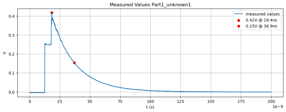
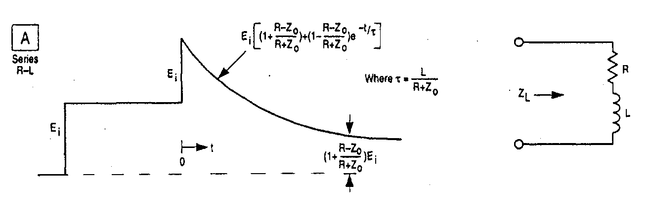
../../_images/time-domain-response_28_0.png

Known:

\(\begin{align} Z_0 &= 50 \\ Ei &= 0.25 \\ V_0 &= 0.4179 \\ \tau &= 18.5 ns \end{align}\)

Solve:

\(\begin{align} 0.4179 &= E_i + E_i\frac{R-Z_0}{R+Z_0} & \rightarrow R &= 254.46 \Omega \\ \tau &= \frac{R+Z_0}{RZ_0}L & \rightarrow L &= 773 nH \end{align}\)

Part1_unknown2

# Calculated Values
#
R = 254.46           # 220 ohms from 'Values of complex loads 2020-v2 better.pdf'
L = 773 *10**(-9)    # 786 nH   from 'Values of complex loads 2020-v2 better.pdf'
Z0 = 50
Ei = 0.25

# Find V0
x0 = 330
V0 = Part1_unknown2[x0][0]
res = 0.05   # resolution = 0.05ns

# Time Constant
V1 = V0 + 0.632 * (2*Ei-V0)  # 0.4349
x1 = np.where((Part1_unknown2>0.43) & (Part1_unknown2<0.44))[0][0]

# Print
print(f'Initial Voltage       = {round(V0,4)}V at t = {round(x0*res,1)}ns')
print(f'System Response 1-1/e = {round(V1,4)}V at t = {round(x1*res,1)}ns')
print(f'Time Response Tau     = {round((x1-x0)*res,1)}ns')

Initial Voltage       = 0.3195V at t = 16.5ns
System Response 1-1/e = 0.4336V at t = 41.0ns
Time Response Tau     = 24.5ns

# Measured Values: Part1_unknown2
#
fig,ax = plt.subplots(figsize=(12,4))
x = np.linspace(0,200*10**(-9),len(Part1_unknown1))
Ures = 0.05
res = 0.05*10**(-9)

# Plot
ax.plot(x,Part1_unknown2,label='measured values')
ax.scatter(x0*res,Part1_unknown2[x0],color='red',label=f'{round(V0,2)}V @ {round(x0*Ures,1)}ns')
ax.scatter(x1*res,Part1_unknown2[x1],color='red',label=f'{round(V1,2)}V @ {round(x1*Ures,1)}ns')

# Labels
ax.ticklabel_format(axis='x',style='sci', scilimits=(-9,-9))
ax.set_title('Measured Values Part1_unknown2')
ax.set_xlabel('t (s)')
ax.set_ylabel('V')
plt.grid(True)
plt.legend(loc='lower right');

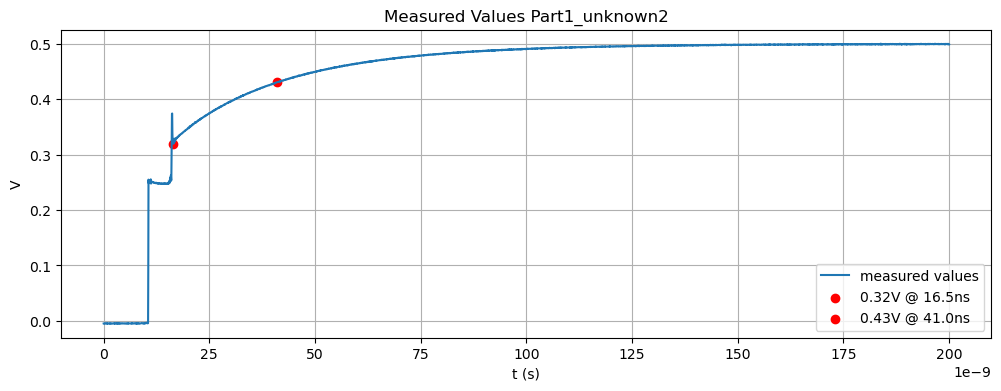
../../_images/time-domain-response_34_0.png

Known:

\(\begin{align} Z_0 &= 50 \\ Ei &= 0.25 \\ V_0 &= 0.3231 \\ \tau &= 24.5ns \end{align}\)

Solve:

\(\begin{align} 0.3231 &= E_i + E_i\frac{R-Z_0}{R+Z_0} & \rightarrow R &= 91.39 \Omega \\ \tau &= (R+Z_0)C & \rightarrow C &= 0.163 nF \end{align}\)

Part1_unknown3

# Find V0 
V0 = max(Part1_unknown3_260ps)[0]
x0 = np.argmax(Part1_unknown3_260ps)

# Time Constant
V1 = V0 - 0.632 * (V0-0.25)  # 0.3068
x1 = np.where((Part1_unknown3_260ps>0.30) & (Part1_unknown3_260ps<0.31))[0][-1]

# Resolution
x,res = np.linspace(0,2.6*10**(-9),len(Part1_unknown3_260ps),endpoint=False,retstep=True)
Ures = res*10**12

# Print
print(f'Initial Voltage       = {round(V0,4)}V at t = {round(x0*Ures,1)}ps')
print(f'System Response 1/e   = {round(V1,4)}V at t = {round(x1*Ures,1)}ps')
print(f'Time Response Tau     = {round((x1-x0)*Ures,1)}ps')

Initial Voltage       = 0.4042V at t = 1114.8ps
System Response 1/e   = 0.3068V at t = 1514.5ps
Time Response Tau     = 399.8ps

# Measured Values: Part1_unknown3
#
fig,ax = plt.subplots(figsize=(12,4))
x,res = np.linspace(0,2.6*10**(-9),len(Part1_unknown3_260ps),endpoint=False,retstep=True)
Ures = res*10**12

# Plot
ax.plot(x,Part1_unknown3_260ps,label='measured values')
ax.scatter(x0*res,Part1_unknown3_260ps[x0],color='red',label=f'{round(V0,2)}V @ {round(x0*Ures,1)}ps')
ax.scatter(x1*res,Part1_unknown3_260ps[x1],color='red',label=f'{round(V1,2)}V @ {round(x1*Ures,1)}ps')

# Labels
ax.ticklabel_format(axis='x',style='sci', scilimits=(-9,-9))
ax.set_title('Measured Values Part1_unknown3')
ax.set_xlabel('t (s)')
ax.set_ylabel('V')
plt.grid(True)
plt.legend();

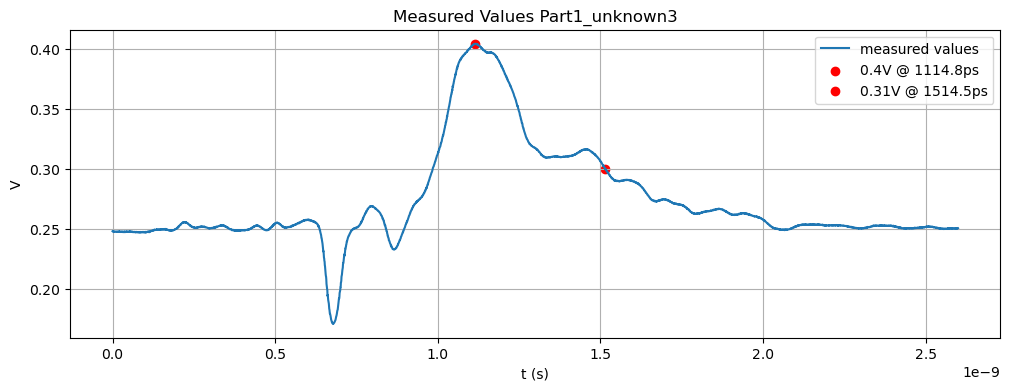
../../_images/time-domain-response_39_0.png

Known:

\(\begin{align} Z_0 &= 50 \\ Ei &= 0.25 \\ V_0 &= 0.4044 \\ \tau &= 399.8 ps \end{align}\)

Solve:

\(\begin{align} E_i &= (1+\frac{R-Z_0}{R+Z_0})E_i & \rightarrow R &= 50 \Omega \\ \tau &= \frac{L}{Z_0+R} & \rightarrow L &= 40 nH \end{align}\)

Uknown Loads Summary

Unknown1: Shunt R-L

	R (Ohms)	L (nH)	C (nF)
measured	254.46	773	-
provided	220	786	-

Unknown2: Series R-C

	R (Ohms)	L (nH)	C (nF)
measured	91.39	-	0.163
provided	100	-	0.184

Unknown3: Series R-L

	R (Ohms)	L (nH)	C (nF)
measured	50	40	-
provided	50	29	-

(4) Small Inductance#

Instructions: characteristics of the input wave form

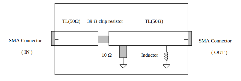
Connect the cable channel 1 and Channel 2 directly as Fig.II-2
Adjust the voltage scale to see the details
Using the THRU measurement, obtain the peak voltage and rise time of the input signal
Read data into PC and use MATLAB or other software to get the peak voltage and rise-time.

Questions

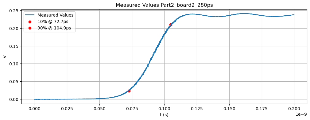
From the measured decay constant, using the relation \(L = R_s \tau\) , compute the inductance of the DUT. If the decay time is too short, skip this part.

Find equivalent circuit \(R_s\)

\(\begin{eqnarray} R_s &=& (50+39)//10//50 \\ R_s &=& (\frac{89 \cdot 10}{89 + 10})//50 \\ R_s &=& 8.99 // 50 \\ R_s &=& (\frac{8.99 \cdot 50}{8.99 + 50}) \\ R_s &=& 7.6 \end{eqnarray}\)

# Find Rise Time

# Median of final 10% elements = 0.2340
fsv = np.median(Part2_calib_ch2_Thu[-int(0.1*len(Part2_calib_ch2_Thu)):])

# 10% value = 0.0234
V0 = 0.1*fsv

# 90% value = 0.2106
V1 = 0.9*fsv

# start
x0 = np.where((Part2_calib_ch2_Thu>0.023) & (Part2_calib_ch2_Thu<0.024))[0][-1]

#end
x1 = np.where((Part2_calib_ch2_Thu>0.210) & (Part2_calib_ch2_Thu<0.211))[0][-1]

# Measured Values: Part2_calib_ch2_Thu
#
fig,ax = plt.subplots(figsize=(12,4))
x,res = np.linspace(0,0.2*10**(-9),len(Part2_calib_ch2_Thu),endpoint=False,retstep=True)
Ures = res*10**12

# Plot
ax.plot(x,Part2_calib_ch2_Thu,label='Measured Values')
ax.scatter(x0*res,Part2_calib_ch2_Thu[x0],color='red',label=f'10% @ {round(x0*Ures,1)}ps')
ax.scatter(x1*res,Part2_calib_ch2_Thu[x1],color='red',label=f'90% @ {round(x1*Ures,1)}ps')

# Labels
ax.ticklabel_format(axis='x',style='sci', scilimits=(-9,-9))
ax.set_title('Measured Values Part2_board2_280ps')
ax.set_xlabel('t (s)')
ax.set_ylabel('V')
plt.grid(True)
plt.legend();

../../_images/time-domain-response_47_0.png

Instructions: The inductance of the DUT

Connect cable 1 to the Test Board port (IN) and cable 2 to the Test Board port (OUT)
Adjust TDR to see the response
Save the measured data

Questions

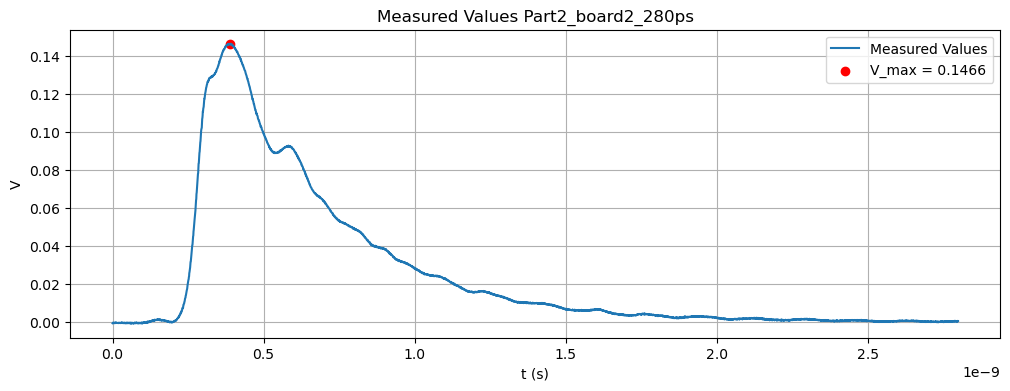
From the measured total area under a response curve, compute the inductance of the DUT

V0 = max(Part2_board2_280ps)[0]
x0 = np.argmax(Part2_board2_280ps)

print(f'V_max is {round(V0,4)}')

V_max is 0.1466

# Area Approximation Part2_board2_280ps Calculation
#
def approx(f,a,b,n,res):
    '''
    Returns the integral approximation of f(x)dx from a to b
    f : continuous waveform
    a : starting point
    b : ending point
    '''
    apprx = 0
    dxs,width = np.linspace(a,b,n,endpoint=False,retstep=True)
    for dx in dxs:
        dx = int(dx)
        midpoint = (f[dx]+f[dx+1])/2 # Use the midpoint approximation
        apprx += width*midpoint # width is 1 nanosecond
    return apprx[0]*res

# Define range and function
a = 250
b = 2400
n = b-a
f = Part2_board2_280ps
x,res = np.linspace(0,2.8*10**(-9),len(Part2_board2_280ps),endpoint=False,retstep=True)
A = approx(f,a,b,n,res)

print(f'Area approximation is {A}')

Area approximation is 6.797642459999998e-11

# Measured Values: Part2_board2_280ps
#
fig,ax = plt.subplots(figsize=(12,4))
x,res = np.linspace(0,2.8*10**(-9),len(Part2_board2_280ps),endpoint=False,retstep=True)

# Plot
ax.plot(x,Part2_board2_280ps,label='Measured Values')
ax.scatter(x0*res,V0,color='red',label=f'V_max = {round(V0,4)}')

# Labels
ax.ticklabel_format(axis='x',style='sci', scilimits=(-9,-9))
ax.set_title('Measured Values Part2_board2_280ps')
ax.set_xlabel('t (s)')
ax.set_ylabel('V')
plt.grid(True)
plt.legend();

../../_images/time-domain-response_51_0.png

# Area Approximation Part2_board2_280ps Plot
#
dxs,width = np.linspace(a,b,n,endpoint=False,retstep=True)

# plot
fig,ax = plt.subplots(figsize=(12,4))
for dx in dxs:
    dx = int(dx)
    midpoint = (f[dx]+f[dx+1])/2
    rect = pch.Rectangle((dx,0),width,midpoint[0],facecolor='#D3D3D3',edgecolor='grey')
    ax.add_artist(rect)
ax.plot(f)
ax.plot(dxs,f[a:b],label=f'area = {round(A,16)}')

# labels
ax.set_xlabel('t')
ax.set_ylabel('V')
ax.set_title('Area Approximation Part2_board2_280ps')
plt.legend();

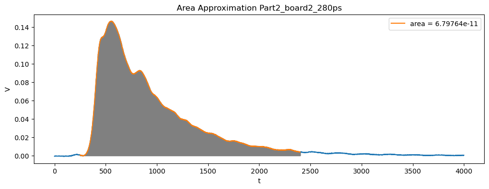
../../_images/time-domain-response_52_0.png

Solve:

\(\begin{eqnarray} V &=& && L \frac{di}{dt} \\ \int V &=& && L \int \frac{di}{dt} \\ \text{area} &=& && L[I(\infty) - I(0)] \\ L &=& && \frac{(\text{area})}{DI} \\ L &=& && \frac{(\text{area})R_s}{DV} \\ L &=& && \frac{6.80 \cdot 10^{-11} \cdot 7.6}{0.1466} \\ L &=& && 3.52 nH \end{eqnarray}\)

Small Inductance Summary

The inductance of the DUT is 3.52 nH.

Kevin Egedy

Time-Domain Analysis

Contents

Time-Domain Analysis#

Objectives#

Constants#

Helpful Equations#

TDS8200 setup#

(1) Measurement of the Verification Devices#

(2) Unmatched Transmission Line#

(3) Unknown Loads#

Part1_unknown1#

(4) Small Inductance#