Shielded-Loop Resonators

Topics

• Measurements of isolated (uncoupled) shielded-loop resonators

• De-embedding the feedline

• Modeling the resonator as an RLC circuit

Useful Equations

\[\begin{split} \begin{align*} \lambda &= \dfrac{u_p}{f} \ (m) \\[0.5em] u_p &= \dfrac{\omega}{\beta} = \dfrac{2l}{\Delta t} \ (m/s) \\[0.5em] \epsilon_r &= \bigg(\dfrac{c}{u_p} \bigg)^2 \\[0.5em] Z_0 &= \sqrt{\dfrac{L'}{C'}} \ (\Omega) \\[0.5em] \beta \ &= \omega \sqrt{\mu \epsilon} = \omega \sqrt{L' C'} \ (rad/m) \\[0.5em] Z_{in} &= Z_0 \dfrac{Z_L + jZ_0 \tan(\beta l)}{Z_0 + jZ_L\tan(\beta l)} \ (\Omega) \end{align*} \end{split}\]

Magnetically-Coupled Resonators

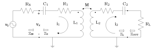
Fig. 35 Schematic of Magnetically-Coupled Resonators

\[ \begin{align*} Z_{in} &= \dfrac{v_x}{i_1} = R_1 + j\bigg(\omega L_1 - \dfrac{1}{\omega C_1} \bigg) + \dfrac{(\omega M)^2}{R_2 + R_L + j\bigg(\omega L_2 - \dfrac{1}{\omega C_2} \bigg)} \end{align*} \]

\[ \begin{align*} Z_{out} = R_2 + j\bigg(\omega L_2 - \dfrac{1}{\omega C_2} \bigg) + \dfrac{(\omega M)^2}{R_1 + R_S + j\bigg(\omega L_1 - \dfrac{1}{\omega C_1} \bigg)} \end{align*} \]

Shielded-Loop Model

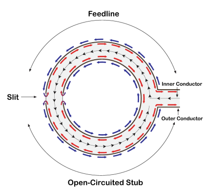
Fig. 36 Shielded-Loop Resonator as Open-Circuited Stub

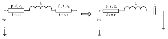
Fig. 37 Open-Circuited Stub Completes Resonant Circuit

Loop capacitance for open-circuited transmission line stub

\[\begin{split} \begin{align*} Z_{in} &= -j Z_0 \cot(\beta l) \bigg|_{\beta l \ll 1} \\[0.5em] Z_{in} &= -j \dfrac{Z_0}{\beta l} \\[0.5em] Z_{in} &= -j \dfrac{\sqrt{L'/C'}}{\omega \sqrt{L' C'} l} \\[0.5em] Z_{in} &= -j \dfrac{1}{\omega C' l} \\[0.5em] C &\approx C' l \end{align*} \end{split}\]

\(C'\) is the per-unit-length capacitance of the tranmission line

Line parameters

\[\begin{split} \begin{align*} C' &= \dfrac{\sqrt{\mu \epsilon}}{Z_0} = \dfrac{\sqrt{\epsilon_r} }{c Z_0} \\[0.5em] C &= \dfrac{\sqrt{\epsilon_r}}{c Z_0} l \\[0.5em] L &= \mu r \bigg[\ln{\bigg(\dfrac{8r}{a_0} \bigg)}-1.75 \bigg], \ {a_0 = \dfrac{d}{4}} \\[0.5em] L &= \mu r \bigg[\ln{\bigg(\dfrac{32r}{d} \bigg)}-1.75 \bigg] \\[0.5em] \beta &= \omega \sqrt{L' C'} = \dfrac{\omega \sqrt{\epsilon_r}}{c} \end{align*} \end{split}\]

• \(\mu\) is the permeability of the surrounding medium

• \(r\) is the radius of the loop

• \(a_0\) is the cross-sectional radius of the loop; defined where rectangular cross-section wire and circular cross-section wire are approximately equal

• \(d\) is the width of the rectangular wire

Resonant Frequency

\[\begin{split} \begin{align*} 0 &= j \omega_0 L + \dfrac{1}{j \omega_0 C} \\[0.5em] \omega_0 &= \dfrac{1}{\sqrt{LC}} \\[0.5em] f_0 &= \dfrac{1}{2\pi \sqrt{LC}} \end{align*} \end{split}\]

Given shielded-loop parameters

Dielectric Properties
Material	Rogers RT/Duroid 5880
Relative Permitivity	\(\epsilon_r = 2.2\)
Loss Tangent	\(\tan \delta = 0.009\)

Conductor Properties
Material	copper
Conductivity	5.8E7 Siemens
Thickness	70 \(\mu\)m

Geometry
Radii	5cm and 9cm
Cross-sectional width	\(d = 15\) mm
Cross-sectional thickness	\(3.32\) mm

Stripline Tranmission Line
Characteristic impedance	\(Z_0 = 50\Omega\)

De-embedding the Feedline

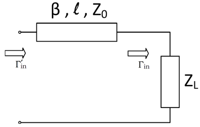
Fig. 38 Effect of Transmission Line on Reflection Coefficient

\[ \begin{align*} \Gamma_{in}' &= \Gamma_{in}e^{-2j \beta l} \end{align*} \]

The insertion of a transmission line with characteristic impedance \(Z_0\) will change the phase of the load input reflection coefficient. Thus, the phase of \(\Gamma_{in}'\) should be increased by 2𝛽𝑙 to find the reflection coefficient of the RLC portion of the loop (\(\Gamma_{in}\)). Note \(\beta\) is frequency dependent so each frequency point must be adjusted by a different phase value.

De-embedding is the process of removing feedline effects.

Characterize the Resonator as an RLC Circuit

E5063A ENA Vector Network Analyzer

Measurements

Loop	Resonant Frequency	Reflection Coefficient \(\Gamma_{in}'(f_0)\)	Phase \(\phi\)
5 cm loop	\(f_0 = 85.7\) MHz
9 cm loop	\(f_0 = 47.4\) MHz

Calculate: Electrical Length

\[ \begin{align*} 2\beta l = (180^{\circ} - \phi)\cdot \dfrac{pi}{180^{\circ}} \end{align*} \]

Loop	\(\beta l\)
5 cm loop
9 cm loop

Finding R

At resonance, the input impedance \(Z_{in}\) is purely real. \(Z_{in} = R_{in} < Z_0.\) Note the input reflection coefficient is purely real and negative.

\[\begin{split} \begin{align*} R = R_{in}(f_0) &= Z_0 \dfrac{1 + \Gamma_{in}}{1 - \Gamma_{in}} \\[0.5em] &= Z_0 \dfrac{1 - |\Gamma_{in}|}{1 + |\Gamma_{in}|} \end{align*} \end{split}\]

Additionally, if the feedline is lossless, then \(|\Gamma_{in}'| = \Gamma_{in}|\).

Finding L and C

To find \(L\) and \(C\), we need measurements at two distinct frequencies.

\[\begin{split} \begin{align*} \omega_a = 2 \pi (f_0 - 2 \text{MHz}) & \ & \omega_b = 2 \pi (f_0 + 2 \text{MHz}) \\[0.5em] \Gamma_a' = \Gamma_{in}'(\omega_a) & \ & \Gamma_b' =\Gamma_{in}'(\omega_b) \\[0.5em] \Gamma_a = \Gamma_a' e^{2j \beta_a l} & \ & \Gamma_b = \Gamma_b' e^{2j \beta_b l} \end{align*} \end{split}\]

Measurements: Reflection Coefficient

Loop	\(\Gamma_{a}'\)	\(\Gamma_{b}'\)
5 cm loop
9 cm loop

Calculate: Electric Length

\[\begin{split} \begin{align*} \beta_a l = \beta l \cdot \bigg(\dfrac{f_0 -2\text{MHz}}{f_0}\bigg) & & \beta_b l = \beta l \cdot \bigg(\dfrac{f_0 +2\text{MHz}}{f_0}\bigg) \\ \end{align*} \end{split}\]

Loop	\(\beta_a l\)	\(\beta_b l\)
5 cm loop
9 cm loop

Using the de-embedded input reflection coefficients, the following is defined

\[\begin{split} \begin{align*} X_a = Im\bigg\{Z_0\dfrac{1+\Gamma_a}{1-\Gamma_a} \bigg\} = \omega_a L - \dfrac{1}{\omega_a C} \\[0.5em] X_b = Im\bigg\{Z_0\dfrac{1+\Gamma_b}{1-\Gamma_b} \bigg\} = \omega_b L - \dfrac{1}{\omega_b C} \end{align*} \end{split}\]

Solving these relations simultaneously results in expressions for \(L\) and \(C\).

\[\begin{split} \begin{align*} C &= \dfrac{\omega_b^2 - \omega_a^2}{\omega_a^2 \omega_b X_b - \omega_b^2 \omega_a X_a} \\[0.5em] L &= \dfrac{\omega_b X_b + \dfrac{1}{C}}{\omega_b^2} \end{align*} \end{split}\]

Q Factor

\[\begin{split} \begin{align*} Q(f_0) = \dfrac{\omega_0 L}{R} &= \dfrac{1}{\omega_0 R C} \\[0.5em] &= \dfrac{\sqrt{LC}}{RC} \\[0.5em] &= \dfrac{1}{R}\sqrt{\dfrac{L}{C}} \end{align*} \end{split}\]

Summary

	\(R \ (\Omega)\)	\(L \ (nH)\)	\(C \ (pF)\)	\(Q\)
5 cm loop
9 cm loop